
- How to add new indicators to existing core layers of a data catalog
- How to add a new date to existing indicators in a data catalog
- How to add data for existing indicators to a new core layer in a data catalog
- How to add data for new indicators to a new core layer in a data catalog
This article is particularly aimed at clients that use the InstantAtlas National Data Service.
Before carrying out any of the steps described below, we recommend that you read the full article to make sure that you have a clear understanding of the entire process. You should make a plan of what you need to do and note down the names that you want your geodatabases, hosted layers and fields to have. Think carefully about these and be consistent, as it may be difficult to change them later once you have created outputs (reports or dashboards) based on the new core layers and data. Contact support@instantatlas.com if you are unsure about anything before you start.
The data loading scenario for this article is the following: Your data catalog contains several core layers, e.g. LSOA, Wards, UTLA, Region and Country. You previously loaded your own Fuel Poverty indicators for a subset of these core layers (LSOA, UTLA, Region and Country) but not for the Ward layer. Now you would like to add data for these indicators for the Ward layer.
Please note that if you use one of the InstantAtlas National Data Services , you will not be able to add data to indicators that are part of the service. You can only add data to indicators you loaded yourself.
To add data into your data catalog, it needs to be saved in your ArcGIS Online account in one or more feature layers . If you want to use the data in either the Report Builder or Dashboard Builder apps, and you wish to see comparison values in the outputs, it is essential that the feature layers contain relationship classes between the core layers and also between the data layers. The Comparison Areas and Relationships page provides further information on this topic. At time of writing it is not possible to create relationship classes within ArcGIS Online so you will need to use either ArcGIS Pro or ArcMap to create the feature layer(s).
To add data to existing indicators for further core layers, you must first locate the feature layer that the existing instances of this indicator are stored in. Data for the same indicator across multiple layers must be saved in the same feature layer in order to be able to create the necessary relationship classes. The easiest way to find the feature layer is to open your data catalog in the Data Catalog Manager, find the indicator and click on the icon. At the top of the dialog you will see the link to the feature service.
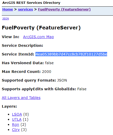
Click this link and you will see the layer description of the feature service. In the bread crumb at the top click on the item one level above. It will be called ‘something (FeatureServer)’.

On the feature server page, find the Service ItemId. Copy it to your clipboard.
Now sign in to your ArcGIS Online account and click on the magnifying glass in the main menu at the top to search for items. Paste the ID from your clipboard into the search field. As a result, you will see the feature layer that contains the fuel poverty indicators.

You can now either export the feature layer to a file geodatabase (open the item’s details page and click Export Data – Export to FGDB) or you can look for the file geodatabase that was used to originally create the feature layer. The latter would save the step of exporting but should only be done, if you are confident that the feature layer has not been changed since it was uploaded.
To find the file geodatabase from which the feature layer was originally created, open the details page for the feature layer and have a look at the Details section on the right underneath the buttons. Follow the link to the file geodatabase listed next to Created from.

From the details page of the File Geodatabase you can download the database using the Download button on the top right-hand side. Browse to the location you downloaded the database to and extract the zip archive.
When you received your master table and metadata table from the Geowise Support Team you would have also been sent a zip archive containing a file geodatabase with the core layers of your data catalog likely called <MyOrganisation>_CoreLayers.zip. If you have not received this, please contact support@instantatlas.com. You will need this file geodatabase to get the Ward layer into the fuel poverty feature layer.
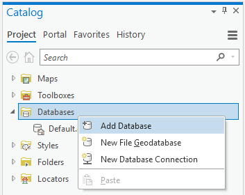
Now open ArcGIS Pro and connect both file geodatabases (the one with the existing fuel poverty indicators and the one with the core layers) to your project. To do this, right-click on Databases in the Catalog Project pane and select Add Database. Then browse to the file geodatabase.
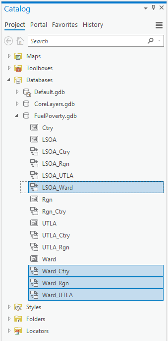
Expand the contents of both databases. You will see that the Ward layer only exists in the core layers database. To copy the layer to the fuel poverty database you should use the Geoprocessing Tool Feature Class to Feature Class. You can drag the Ward layer from the base core layers geodatabase into the Input Features field and drag the fuel poverty file geodatabase into the Output Location field. Give the Output Feature Class the same name as the input layer, in this case Ward.

Click Run and the Ward layer will be added to your fuel poverty database.
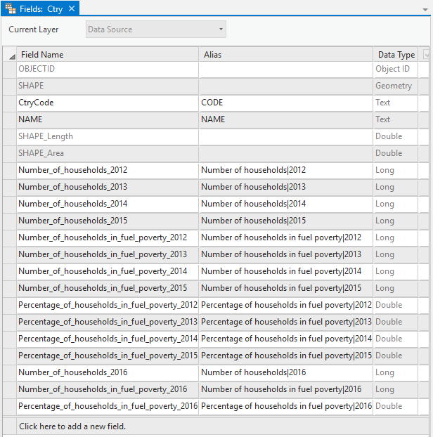
If you right-click on one of the data layers in your fuel poverty database (any layer except for the new Ward layer) and click on Design – Fields you will see the fields that are currently part of this layer. You can see the required field format for indicators with multiple dates in the Alias column: the indicator name needs to be followed by a pipe character ‘|’ and the date.
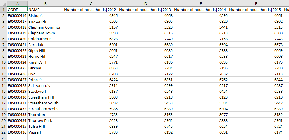
Before you can add the data for Wards, you should ensure that it is correctly formatted. You will need one CSV file per data layer (in this example it would be just one file for the Ward layer), containing a column with the feature codes. These codes need to match the code column in the respective data layer in the file geodatabase so that you can connect the data to the data layers. The first row needs to contain the column headers. The column headers of the indicator columns need to match those of the existing fields of the other data layers, so that the Data Catalog Manager will understand that these are the same indicators, just for different layers.
If you wish to add data for multiple existing core layers at the same time, you can do this in additional CSV files, applying the same rules.
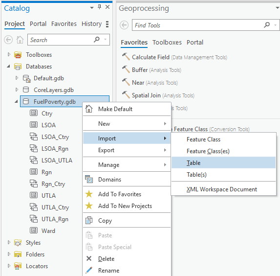
Now you can load the CSV file into your File Geodatabase as a table. To do this, right-click on the database and select Import – Table.
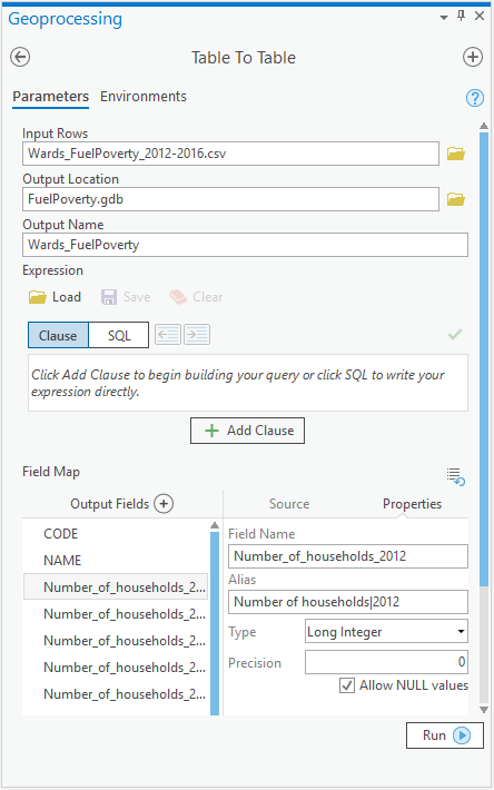
The Geoprocessing Tool Table To Table opens. Select the CSV file as Input Rows and give it a suitable Output Name (this table is just a temporary item in the database so the name does not matter).
It is now important to check that all output fields are loaded in the Field Map with their correct data type. Click on the first field and select Properties. The Type property is derived from the first value of the field so you should check that it is correct for each field and adjust if necessary. For example, if you add a rate indicator and the first value of the column happens to be an integer value, the whole field will be imported as Long Integer, stripping the decimal places from all other values of the column.
Click Run to import the data. When complete, the table will appear within your database in the Catalog Project pane. To check whether the import was successful you can add the table to a map. You can open the table and see the values if you right-click on the entry in the Content pane and select Open.
Repeat the data loading steps for each of the CSV files if you are loading data for multiple layers at a time.
The next step is to join the data from the imported table to the data layer. In the Geoprocessing pane, click the Back icon and find the tool called Join Field. Choose your data layer as the Input Table (you can drag and drop it from the Catalog Project pane) and the imported table as the Join Table. Select the matching code fields as Input and Output Join Field.
Open the Join Fields drop down and toggle all checkboxes to select all fields. There is a button at the bottom of the drop-down list that does this for you. You may wish to uncheck the columns containing the feature code and names as they will already exist in the data layer.

Then click Add and Run to join the selected fields to the data layer. The layer will automatically be added to your map if you have one open. You should check that the join was successful by opening the attribute table of the layer (right-click on the layer in the Content pane and select Attribute Table).
Once the join is complete you can delete the temporary table you imported from the CSV file from the database (right-click on the item in the Catalog Project pane and select Delete).
To be able to see comparison geographies in a dashboard or report created with the InstantAtlas Dashboard Builder or InstantAtlas Report Builder apps respectively you will need relationship classes set up between the data layers in the underlying feature services. So far you have added the Ward layer to your fuel poverty file geodatabase, and have joined the data to the layer, but there are no relationship classes to other data layers yet.
To create relationship classes, find the Geoprocessing Tool Create Relationship Class. Select the higher data layer as Origin Table (e.g. UTLA) and the lower data layer as Destination Table (e.g. Ward). You can again drag and drop the layers from the fuel poverty database in the Catalog Project pane. The remaining properties will automatically be filled with default values. The ones you should change are:
Output Relationship Class: change the name to follow this pattern ‘<destination layer>_<origin layer>’ e.g. Ward_UTLA. Please note that this is contrary to what ArcGIS Pro suggests by default. You can add another underscore followed by a feature service identifier to the relationship class name e.g. Ward_UTLA_fuelpov.
Cardinality: change this to be One to many (1:M).
Origin Primary Key: Select the feature code field in the origin table.
Origin Foreign Key: Select the field in the destination table containing the matching codes from the origin table code field.

Leave all other settings at their default values and click Run. The relationship class will appear in your database. Create the relationship classes to other data layers in the same way.
Now close ArcGIS Pro and browse to your file geodatabase containing the fuel poverty data in Windows explorer. Zip it and ensure that the file name is the same as the zip archive you downloaded earlier from ArcGIS Online. If the original zip file is saved in the same folder and you want to keep it as a backup, you may wish to rename it first.
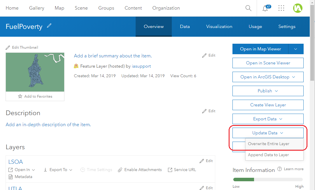
Back in ArcGIS Online, open the details page of the Fuel Poverty feature layer (not the related file geodatabase item) and click on the Update Data button on the right. Then select the option Overwrite Entire Layer.
Browse to your zipped file geodatabase (the one you just added the Ward data to) and click Overwrite. This will update the feature layer as well as the related file geodatabase.
Now you should sign in to https://hub.instantatlas.com/ and click on the Manage Catalog button. You should see your Data Catalog with Core Layers and Data Model for each layer.
Select the Ward layer and open the tree to the theme that contains the fuel poverty indicators in the other layers. Select the theme and click on the Add Indicator Connection button.

In the dialog that opens, select the feature layer you updated in ArcGIS Online. If there are many feature layers in your organisation’s account you can use the search field or sort options at the bottom of the dialog to help you find the right one. Click Choose. Now select the correct data layer that corresponds to the active core layer in your data catalog and click OK. You will see a dialog with the fields you can add as indicators. Fields that have been formatted with a pipe character followed by a date are automatically recognised as different dates for the same indicator and will be pre-selected.
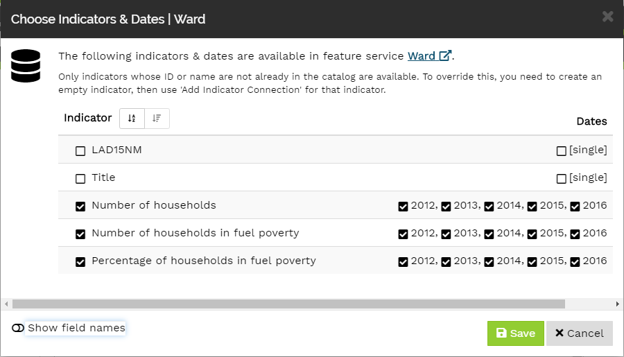
Select the indicator(s) you wish to add and click Save. The indicators should then appear in your data model.
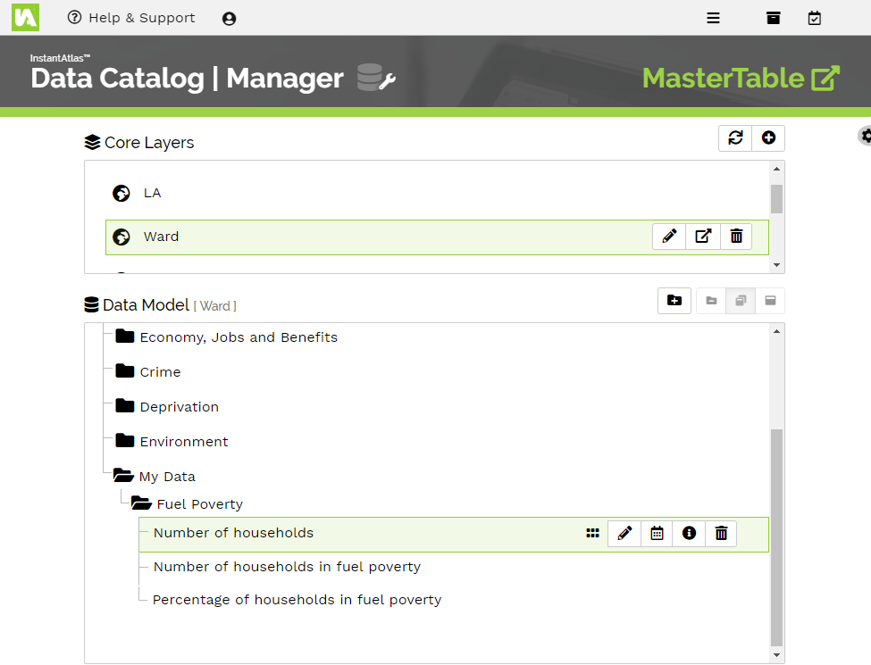
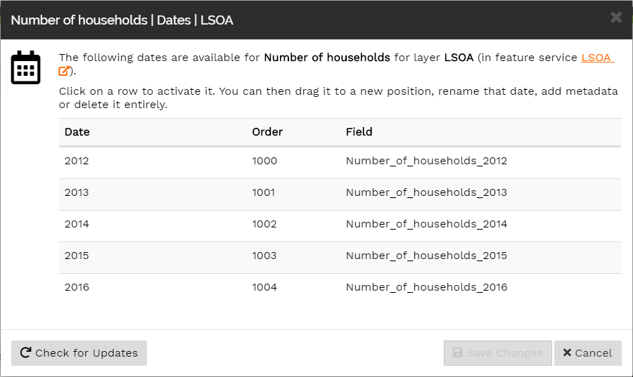
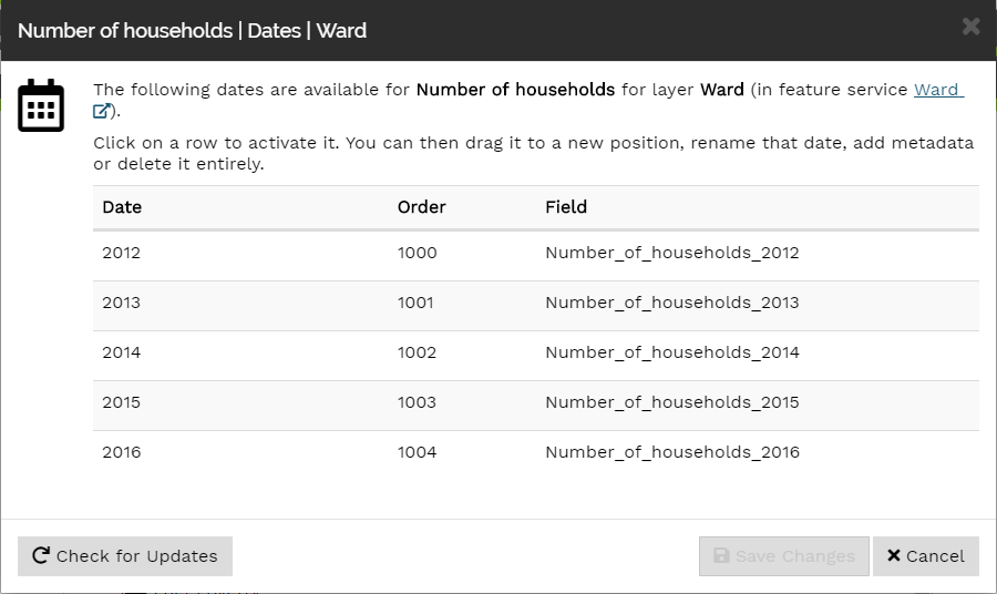
To check that the import was successful, you can click on the icon to see the instances (dates) belonging to the indicator.
If you are adding data for multiple core layers at a time you can now import the indicators for the other core layers in the same way.
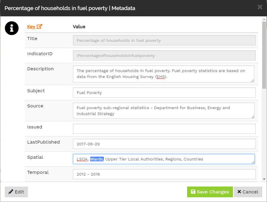
You may wish to update the ‘Spatial’ metadata key (and maybe others) for the indicators to add the new core layer to the list. You can do this by clicking the icon and then clicking on the Edit button.
If you have a large number of indicators, adding metadata through the Data Catalog Manager interface may not be the most efficient method. As an alternative, you can create a CSV file containing the metadata for your new indicators and append it to your metadata table. Please contact support@instantatlas.com for information on how to do this.