Web Map Builder uses smartMapping module(s) from API throughout
Web Map Builder now has a new option to allow proportional symbols for count data (user option). This option is available from the ellipsis menu in the top right corner
Inspector now shows warning messages when Item_Order is missing for an Indicator in the master table
Web Map Builder now handles categoric data gracefully
The Data Catalog Manager pre-checks for new core layers in hosted tables to ensure that updates stay in sync
The Data Catalog Manager disables buttons in the UI that trigger an update whilst another update is still processing
Minor UI cleanup around dialogs and buttons
Bug fixes:
Web Map Builder will now exclude data where all values are null from the map – previously this was causing an error dialog to appear
Web Map Builder how handles Feature Collections properly when opening an existing web map – previously this was generating a JSON error
Metadata page now falls back to using the standard metadata table if there is not one defined within the targeted master table
The first step is to sign in to Report Builder. From the Data Catalog Hub homepage click Report Builder (you must have taken a trial of this app from the ArcGIS Marketplace).
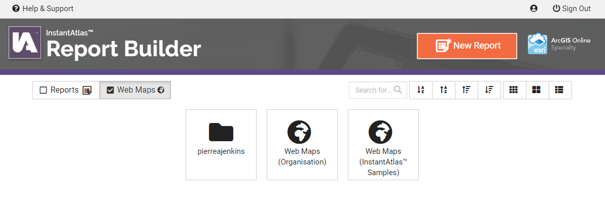
Once in Report Builder, select the Web Maps checkbox in the middle of the page. Then click the Web Maps (InstantAtlas Samples) folder below.
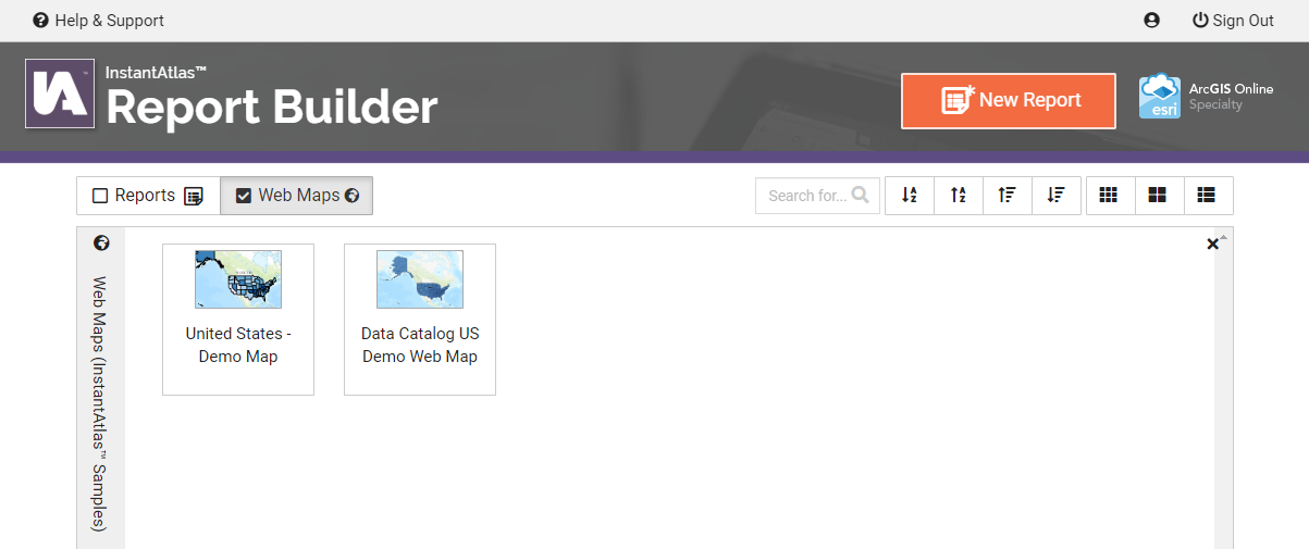
You should see a web map in this folder called Data Catalog US Demo Web Map. That starting point for every InstantAtlas report is a web map. Hover the web map with your mouse pointer and click the Page icon (the middle icon of the three) to create a report based on that web map.
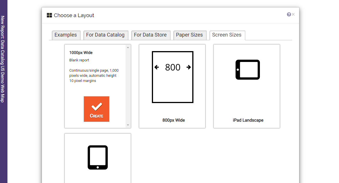
Select the first layout option.
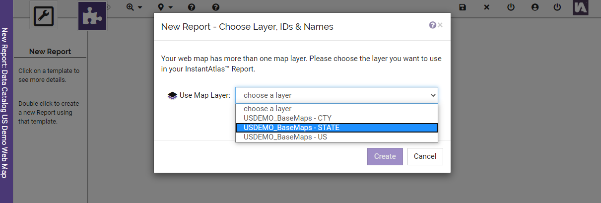
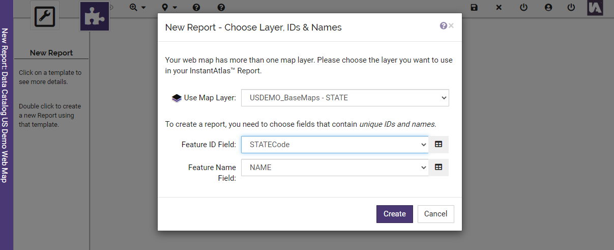
Select the layer you wish to create a report for – County, State or US.
Then select the fields from the layer that contain the IDs and the names of the features in the layer. These are:
County – CtyCode, NAME
State – StateCode, NAME
US – USCode, NAME
In the example shown below the State layer has been chosen.
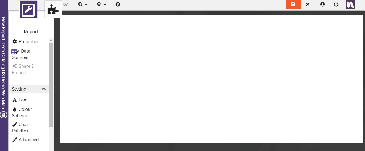
The report will be created and you will be presented with a blank page.
Attaching the data catalog as a data source
You will now see how to attach a data catalog as a data source to a report in Report Builder.
Click the Report Settings and Actions button in the top left-hand corner of the screen. Then click Data Sources.
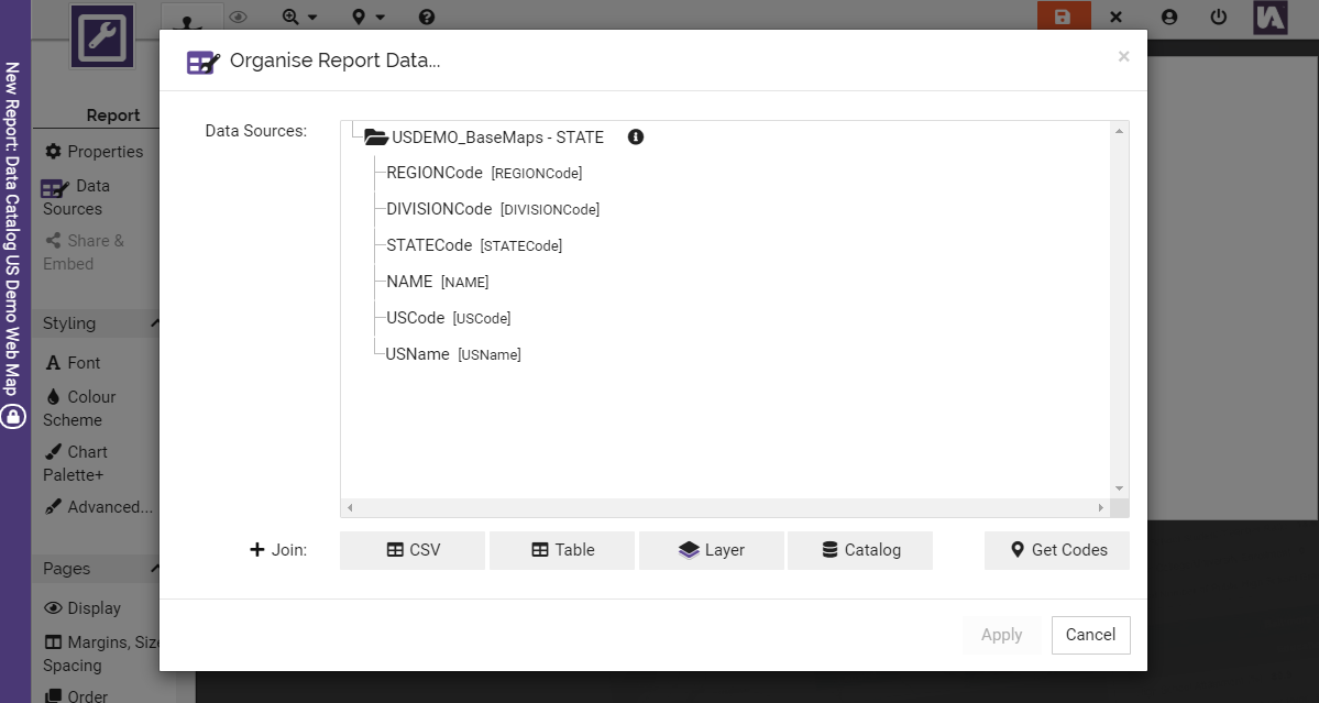
Click the Catalog button and then click Choose Table.
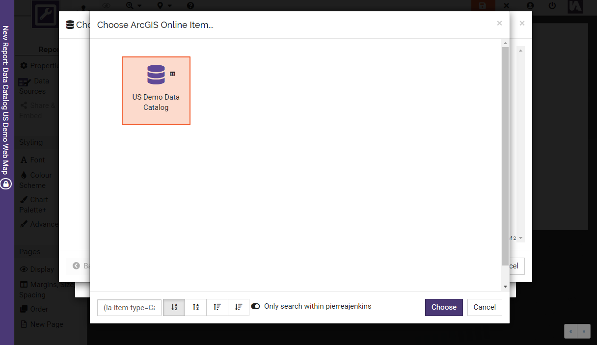
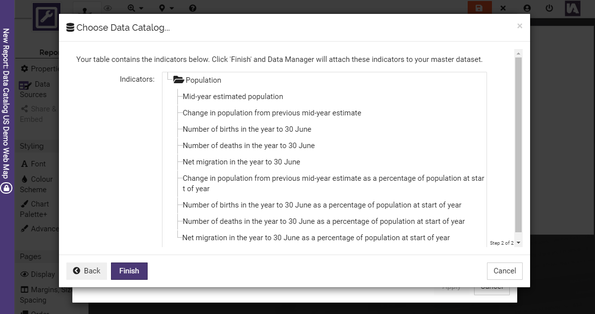
Click on the catalog you created with the US demo data to select it. Then click Choose and Next.
Click the Finish button.
You have now connected the data catalog to the report as a data source.
Displaying the data catalog data in the report
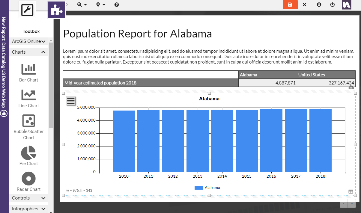
You can now click the Widgets button in the top left-hand corner of the page to start dragging widgets onto the report page. Once you have dragged a widget onto the page, you can edit the widget properties, click the Data tab and select indicators from the data catalog.
You may have just taken out a trial of the Data Catalog app in the ArcGIS Marketplace and are wondering what this app is all about. Alternatively, you or the administrator of your organisational ArcGIS Online account may have purchased a subscription of the Data Catalog app and you are now wondering where to start. This tutorial will give you an overview of the purpose and main features of the Data Catalog.
The Data Catalog app in the ArcGIS Marketplace actually gives you access to four related apps that can be accessed through the InstantAtlas Data Catalog | Hub. These are (click on each item to see a short description):
Data Catalog | Manager
The purpose of the Data Catalog Manager is to organise data from different feature services into a logical structure that will help you and your colleagues to quickly find the data you are looking for to use it in Web Maps or in the InstantAtlas Report Builder or Dashboard Builder apps.
Data Catalog | Inspector
The Inspector allows you to check whether your data catalog contains any errors. It also gives an overview over how many core layers, themes, indicators, instances (dates) and relationships exist in your data catalog.
Data Catalog | Explorer
The Explorer lists all of the indicators of your data catalog, together with their metadata and the core layers they exist for. The explorer contains a search tool, filter and download options and a way to view the data as a table or on a map.
Data Catalog | Web Map Builder
The Web Map Builder allows you to create a webmap containing one or more data layers from your data catalog.
Creating a new data catalog with population data
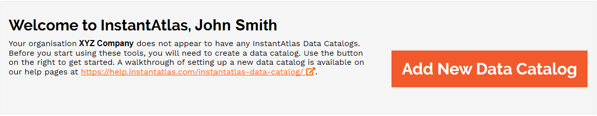
To use each of these apps you will need a valid InstantAtlas data catalog in your ArcGIS Online account. Assuming you are new to the Data Catalog app, it is likely that you don’t have an InstantAtlas data catalog yet. The homepage of the Hub will detect this and display a welcome text together with a big orange button labelled Add New Data Catalog at the top right-hand side.
Click this button and you will be directed to the Add New Catalog page.
If your organisation already has an InstantAtlas data catalog, you won’t see the welcome text and the orange Add New Data Catalog button. If you still wish to follow this tutorial to get familiar with the Data Catalog apps, you can force the creation of a new catalog by clicking on Manage Catalog in the hub homepage and then changing the URL in your browser from /manager?item=<itemid> to /manager?catalog=new.
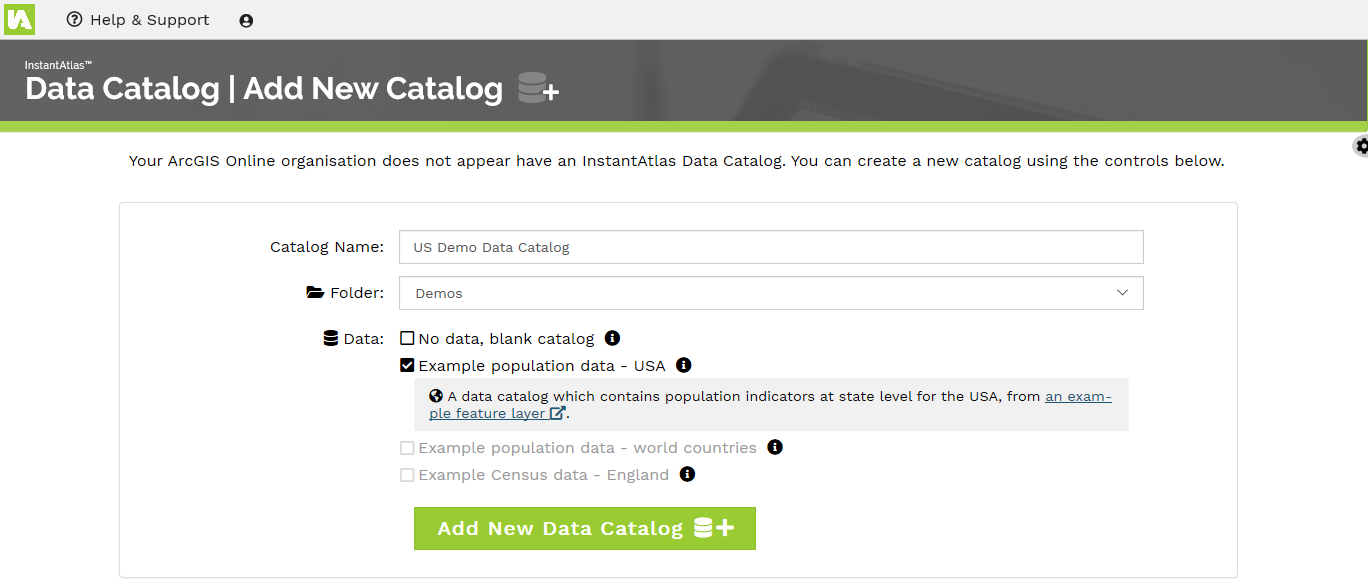
On the Add New Catalog page, enter a suitable name for your new data catalog and select the folder you want it to be saved in. Then, under Data, select Example population data – USA. Now click on the button Add New Data Catalog.
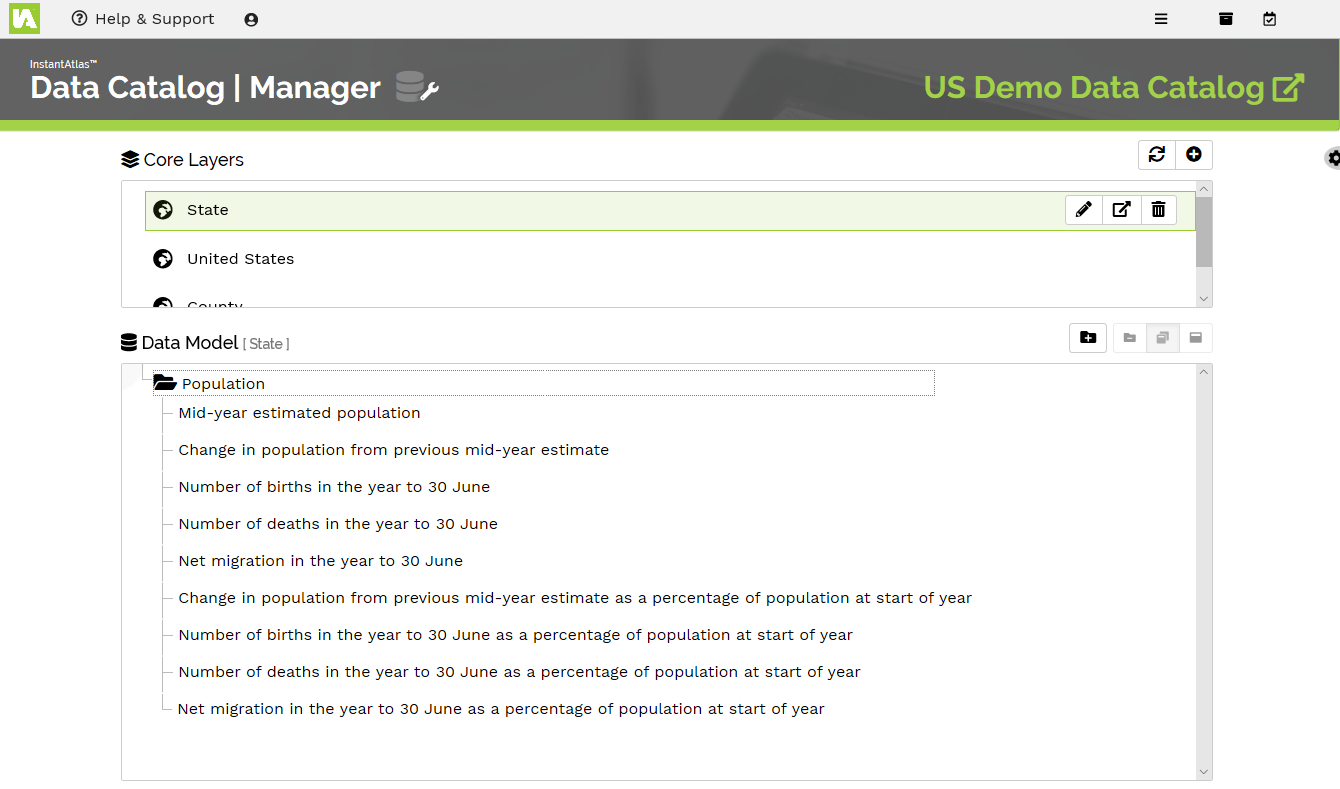
The new data catalog is created in the specified folder and a bar will indicate progress. Once finished, the Data Catalog|Manager will open showing the content of the data catalog.
At the top of the screen you will see a list of Core Layers. A core layer is a feature layer that represents the geographical features for which data is to be viewed. In this example dataset, there are three core layers: County, State and United States.
Below the core layers you will see the Data Model for the selected core layer. A data model consists of themes, sub-themes and indicators in a tree structure.
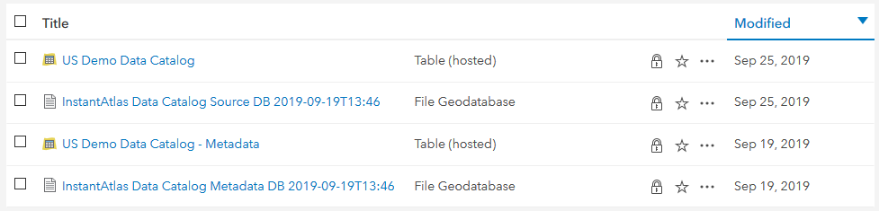
Before editing the data model in the Data Catalog Manager, you may want to have a look at your ArcGIS Online content, particularly the folder you specified when creating the new data catalog. You will see two new hosted tables together with their relating file geodatabases.
The table with the same name as your new data catalog is called the master table. Open the item’s details page and click on Data in the blue menu (top left-hand side). This table contains the definition of the core layers and data model with its themes, indicators and instances. If you scroll to the right you will find the Service_URL field containing the references to the relevant feature services.
The second new table in your folder contains the metadata for the indicators / instances in the data catalog.
Creating sub-themes and moving indicators
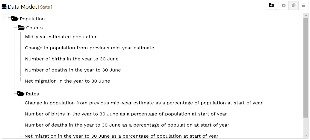
Back in the Data Catalog Manager, explore the data model of the US example population data catalog. Initially it only contains one theme called Population and a number of indicators within this theme (click on the folder name to expand its contents).
Different core layers can contain different indicators; however, the theme structure is the same across all core layers and hence only needs to be defined for one of them. Let’s create two sub-themes within the Population theme and move the existing indicators into the two new themes.
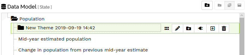
To create a sub-theme, select the parent theme (in this example Population) and click on the Add Theme button. A new folder will appear within the Population folder called New Theme <yyyy-mm-dd hh:ss>, where <yyyy-mm-dd hh:ss> is being replaced by the date and time stamp of the theme creation.
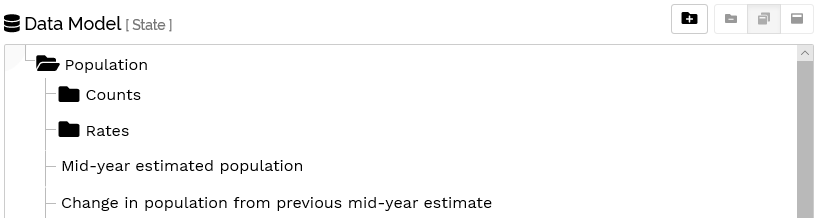
To rename the theme, select it, so that it is highlighted and click on the button and enter Counts as the new theme name. Select the button to submit the changes. In the same way create a second sub-theme within the Population theme called Rates.
Next you will move the indicators that contain the word ‘percentage’ in the indicator name into the Rates sub-theme. The other indicators are to be moved into the Counts sub-theme. To move an indicator, select it and use the button to drag and drop the indicator into the respective sub-theme folder. A green plus icon needs to appear to the left of the folder you wish to move the indicator into before you release your mouse button. The data model will refresh after every move to show the changes.
If you have moved the indicators whilst having either the State or the United States core layer active you should now select the County core layer. You will find additional indicators in the County core layer that do not exist in the other two. Move these indicators into their respective sub-themes as well.
You may have noticed that when you make a change to an indicator (e.g. its position but it applies to the name as well) this is reflected no matter which core layer is selected above.
Adding income indicators from a second feature service
Currently the data catalog only contains data from one single feature service. One of the benefits of the Data Catalog Manager is that it is possible to manage and organise data from multiple different feature services that might be saved in different ArcGIS Online accounts. To demonstrate this, let’s assume you have some income related indicators in a second feature service and you wish to add them to your data model.
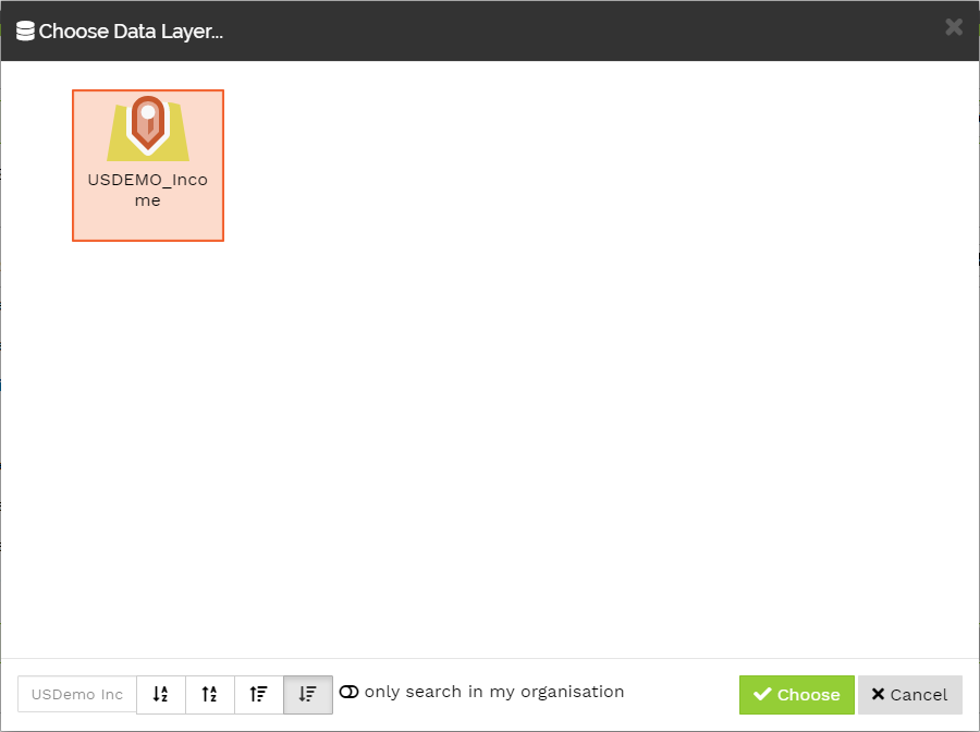
As a first step, create a new root theme by clicking on the Add Theme button at the top right-hand side of the data model. Rename this theme to Income and create two sub-themes, one called Households and the other called Families. With the Households theme selected, click on the Add Indicator Connection button. At the bottom of the Choose Data Layer… dialog switch the option only search in my organisation off. In the search field at the bottom left hand side type USDemo Income. Select the Feature Service called USDEMO_Income and click Choose.
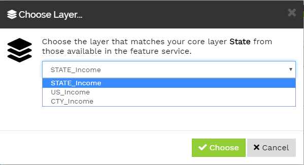
In the Choose Layer… dialog that opens, select the layer from the drop-down list that corresponds to the active core layer in your data catalog. For example if you have the core layer State active you should pick STATE_Income from the drop-down list. Then click the Choose button.
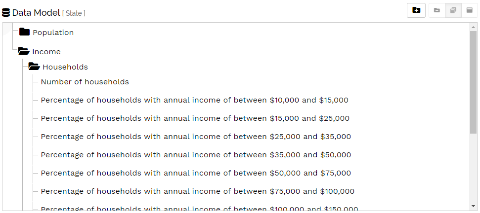
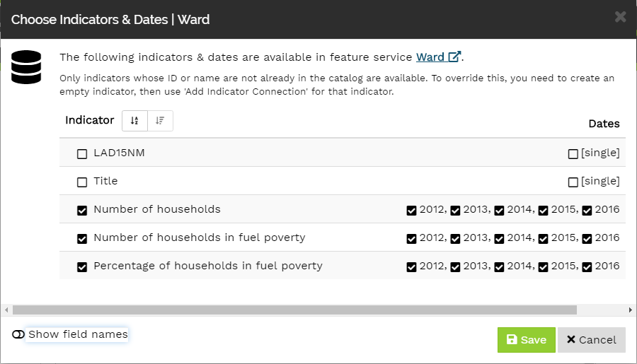
In the Choose Indicators & Dates dialog, untick the checkbox of all indicators that are not related to households. Leave all date checkboxes ticked. Then click the Save button.
As a result, you will see all household income related indicators listed in the Households sub-theme within the Income theme.
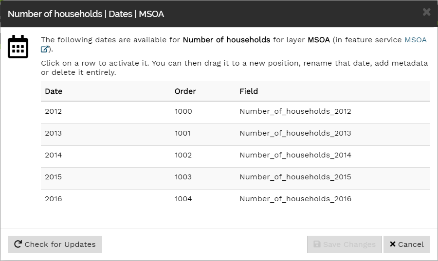
You can check if the references to the data fields from the feature service were generated successfully by selecting one of the indicators and clicking the Dates button. The dialog that opens shows all dates for that indicator together with their field names from the feature service. You can also find the link to the feature service at the top of the dialog.
Please note that the data catalog stores only references to the feature services holding the data – the data values themselves are not imported into the master table.
Similar to adding the household income indicators, you should now add the indicators related to family income into the Families sub-theme.
Adding indicators has to be done for each core layer separately, so you may want to add the available income indicators into the relevant theme for the other two core layers.
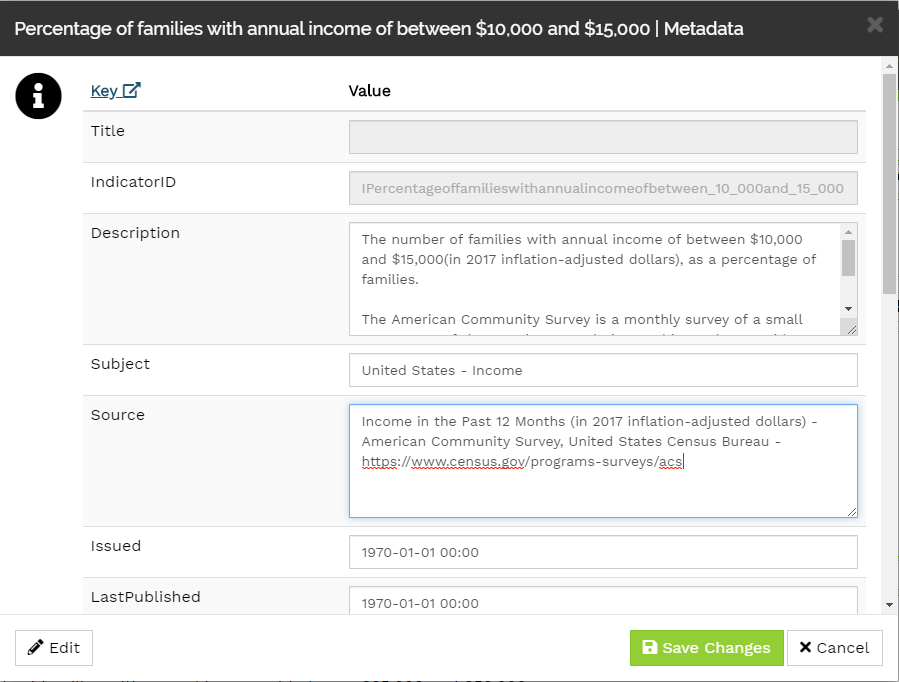
If you wish to add metadata for your new indicators, this can be done by clicking on the button of a particular indicator. You will see the list of available metadata items with the IndicatorID already filled in. Click on the Edit button at the bottom left-hand side to enter metadata information. The Title will be added as soon as you click on the Save Changes button (Title and IndicatorID cannot be changed via this dialog).
If you have a large number of indicators, adding metadata through the Data Catalog Manager interface may not be the most efficient method. As an alternative, you can create a CSV file containing the metadata for your new indicators and append it to your metadata table within ArcGIS Online.
Checking the data catalog using the Inspector
Once you have added all indicators for all core layers to the data catalog, you can now use the Data Catalog|Inspector to check that the data catalog is valid.
There are two ways to access the inspector: You can return to the Hub homepage by clicking the logo at the top left-hand corner of the screen and then select Inspect Catalog. Alternatively, click on the cogwheel icon on the right-hand side of the page. This opens a wheel from where the other apps – including the Inspector – can be accessed.
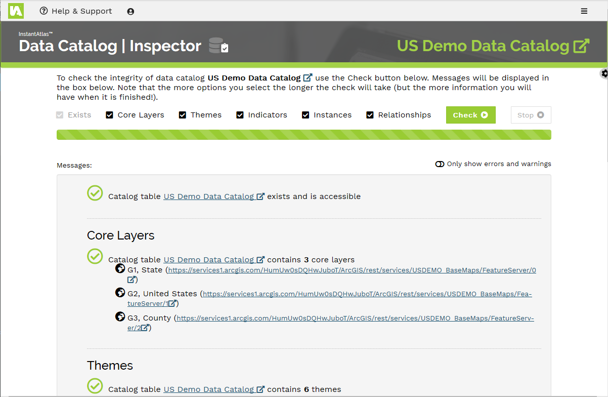
The Inspector allows you to check the integrity of your data catalog. You can choose which items (core layers, themes, indicators, instances and relationships) of the data catalog to include in the inspection. Once you made your selection, click the green Check button. Messages will be displayed in the box below.
A green circled tick indicates that no issues were found with this element. If you see warnings and/or errors these should be attended to as they could have an impact on your data showing correctly in a web map or an InstantAtlas report. If you need assistance in solving any issues, please get in touch with support@instantatlas.com.
Browsing the data using the Explorer
There are two ways to access the Explorer: You can return to the Hub homepage by clicking the logo at the top left-hand corner of the screen and then select Explore Catalog. Alternatively, click on the cogwheel icon on the right-hand side of the page. This opens a wheel from where the other apps – including the Explorer – can be accessed.
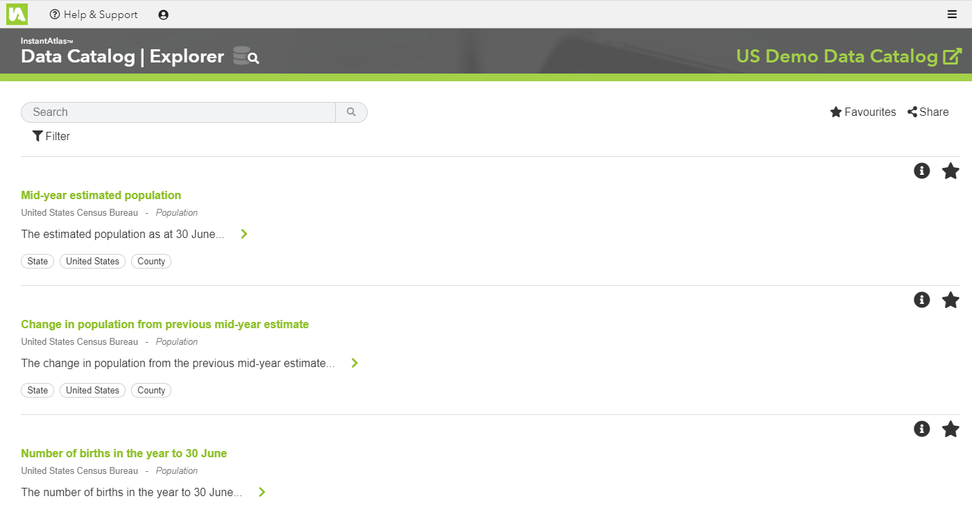
The explorer allows you to search for a particular indicator using the search field and/or filter the list of indicators by theme/geography/publisher.
Click on an indicator and then use the tabs to view metadata or view the data in a table, map or chart. There is the option to download the data (CSV) from the Table tab.
Creating a web map using the Web Map Builder
The Web Map Builder allows you to quickly create a web map using one or more of the indicators in your data catalog.
There are two ways to access the Web Map Builder: You can return to the Hub homepage by clicking the logo at the top left-hand corner of the screen and then select Build a Web Map. Alternatively, click on the cogwheel icon at the right border of the page. This opens a wheel from where the other apps – including the Web Map Builder – can be accessed.
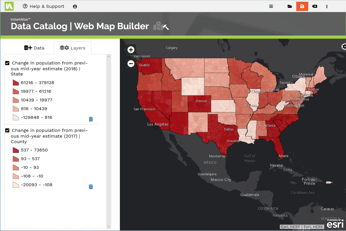
On the left-hand side, you can see the data model of your data catalog in the Data tab. Expand the themes to see the indicators. At the bottom you can change the active core layer. You can add an indicator to the map on the right by clicking on one of the plus icons. The icon adds the selected indicator for the active core layer whilst the icon adds the indicator for all available layers. After you have added one or more indicators, switch to the Layers tab where you can review your selection and if necessary remove layers again.
Once you are happy with your selection click the orange button to save your web map. More information is available on the Web Map Builder help page.
Please note that the Web Map Builder allows you to create a quick starting point for a web map. Its purpose is not to replicate all of the functionality of the ArcGIS Online Map Viewer so for any further changes to the appearance and functionality of your web map you should continue editing it in ArcGIS Online.
What’s next?
Congratulations, you have now completed this introduction tutorial. As a next step we recommend that you have a look at the Data Catalog help pages. You will need to read these carefully if you wish to add further data to your catalog, in order to understand the rules and requirements for the feature services containing the data. If you have any questions that have not been answered yet or if you get stuck in creating your own data catalog, please feel free to contact support@instantatlas.com.
Improved update process for indicators supplied by the InstantAtlas National Data Service but referenced in a customer-managed catalog/master table.
Improved (more fine-grained) error checking in the Inspector tool
New “Repair” functionality in the Inspector tool to allow repair of common errors
Minor UI updates
Bug fixes:
Fixes for issues in the Manager tool that prevented update of InstantAtlas National Data Service indicators and/or caused duplicate indicators and themes in the customer-managed table.
This version is a major release designed to improve the user experience, address a number of bugs, deliver significant speed improvements and to add support for ArcGIS Enterprise/Portal alongside ArcGIS Online.
New features
The Web Map Builder tool can now produce maps with multiple time-specific layers per indicator.
The Manager tool can support indicators that belong to more than one theme.
The Manager and Explorer tools support metadata at both the indicator and instance (indicator, date, geography) level.
An Explorer app (for sharing the contents of your catalog with anonymous users) can now be configured to filter to a specified root level theme in your catalog i.e. to exclude data under other root level themes.
The Inspector tool now has improved service validation, checking that the services, layers, relationships and fields within your data catalog are correctly set up and consistent.
Bug fixes
Drag-and-drop editing in the Manager tool has been completely rebuilt to offer improved consistency and performance.
Fix for viewing the Explorer app in Internet Explorer 11
Before carrying out any of the steps described below, we recommend that you read the full article to make sure that you have a clear understanding of the entire process. You should make a plan of what you need to do and note down the names that you want your geodatabases, hosted layers and fields to have. Think carefully about these and be consistent, as it may be difficult to change them later once you have created outputs (reports or dashboards) based on the new core layers and data. Contact support@instantatlas.com if you are unsure about anything before you start.
For this example, let’s assume that you would like to load data about licenced homes of multiple occupancy. You have a shapefile containing the point locations of these homes and you have a CSV file with the related indicators. Neither the indicators nor the layer exists in your data catalog yet.
To load new indicators into your data catalog, the data needs to be saved in your ArcGIS Online account as one or more feature layers . If you want to use the data in either the Report Builder or Dashboard Builder apps, and you wish to see comparison values in the outputs, it is essential that the feature layers contain relationship classes between the core layers and also between the data layers. The Comparison Areas and Relationships page provides further information on this topic. At time of writing it is not possible to create relationship classes within ArcGIS Online so you will need to use either ArcGIS Pro or ArcMap to create the feature layer(s).
When you received your master table and metadata table from the Geowise Support Team you would have also been sent a zip archive containing a file geodatabase with the core layers of your data catalog, likely called <MyOrganisation>_CoreLayers.zip. If you have not received this, please contact support@instantatlas.com. This file geodatabase is a good starting point as it already contains the relationship classes between the core layers. You should extract the zip archive and take a copy of the file geodatabase. Keep the original one as a reference and rename the copy to for example <MyOrganisation>_CoreLayers_plusCustom.gdb.
Please note: We suggest that you add all of your custom core layers into the same file geodatabase, so if you are already using a feature layer called <MyOrganisation>_CoreLayers_plusCustom.gdb (or similar) in your data catalog you should find it in ArcGIS Online and download the respective file geodatabase.
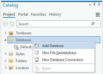
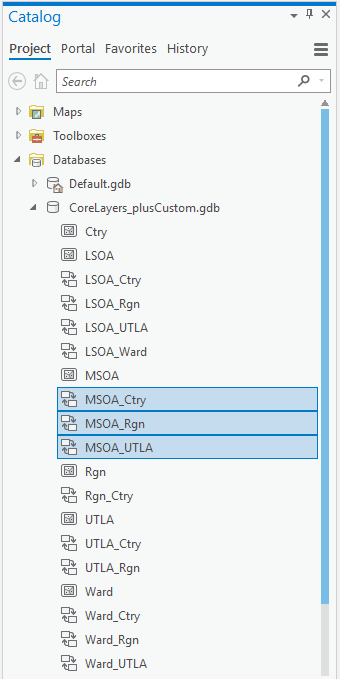
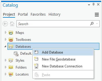
Now connect this file geodatabase to your ArcGIS Pro project. To do this, right-click on Databases in the Catalog Project pane and select Add Database. Then browse to the file geodatabase.
Expand the contents of the database and you will see the core layers of your data catalog and the relationship classes between them.
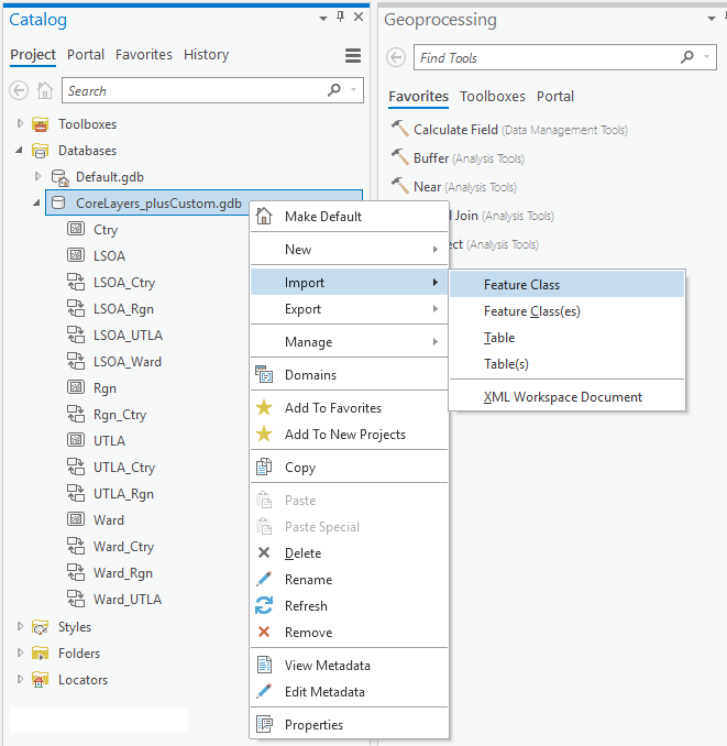
Firstly, you need to add the shapefile for your new core layer to the database with your core layers. To do this, right-click on the database name in the Catalog Project pane and select Import – Feature Class.
For the Input Features browse to the shapefile containing the new layer, then enter a suitable Output Feature Class name (e.g. HMO) and click Run.
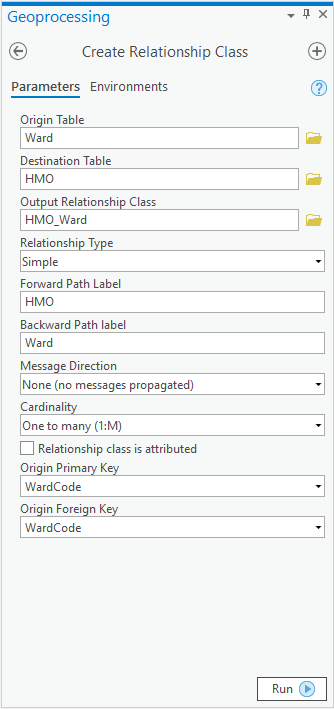
Now add the relationship classes between the new layer and any other layers that you may wish to see as comparison values in Dashboard Builder or Report Builder outputs. You will have to provide/calculate the indicator values for these comparison layers yourself as the apps do not automatically aggregate the data for you. It is assumed that your shapefile contains the necessary lookup fields i.e. a column with the matching codes for each core layer that you want it to relate to. To create relationship classes, find the Geoprocessing Tool Create Relationship Class. Select the higher geography layer as Origin Table (e.g. Ward) and lower geography layer as Destination Table (e.g. HMO). You can drag and drop the layers from the database in the Catalog Project pane. The remaining properties will automatically get filled with default values. The ones you should change are:
Output Relationship Class: change the name to follow this pattern ‘<destination layer>_<origin layer>’ e.g. HMO_Ward. Please note that this is contrary to what ArcGIS Pro suggests by default!
Cardinality: change this to be One to many (1:M).
Origin Primary Key: Select the feature code field in the origin table.
Origin Foreign Key: Select the field in the destination table containing the matching codes from the origin table code field.
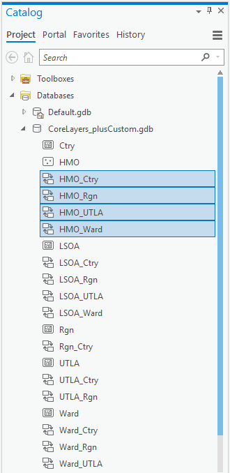
Leave all other settings at their default values and click Run. The relationship class will appear in your database. Create the relationship classes to other core layers in the same way.
If you wish to add more than one new core layer to your data catalog, simply repeat the steps of importing a shapefile and creating the relevant relationship classes.
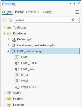
Once the new core layer and all relationship classes have been added, browse to your file geodatabase in Windows explorer and take a copy of it. Rename the copy so that the name describes the data you wish to load; for this example, this could be HMO_indicators.gdb. Now connect this file geodatabase to your ArcGIS Pro project.
You will see the same layers and relationship classes as in your core layers database. Delete any layers that you do not have data for to simplify the database. For this example, the HMO indicators only exist for the HMO layer and can be aggregated to Ward and UTLA level. Therefore, you can delete the LSOA, Rgn and Ctry layers. This will automatically delete all related relationship classes as well. The database now only contains the three layers you would like to load data for, as well as their relationship classes. As you want to add data to these layers, you no longer call them core layers but data layers.
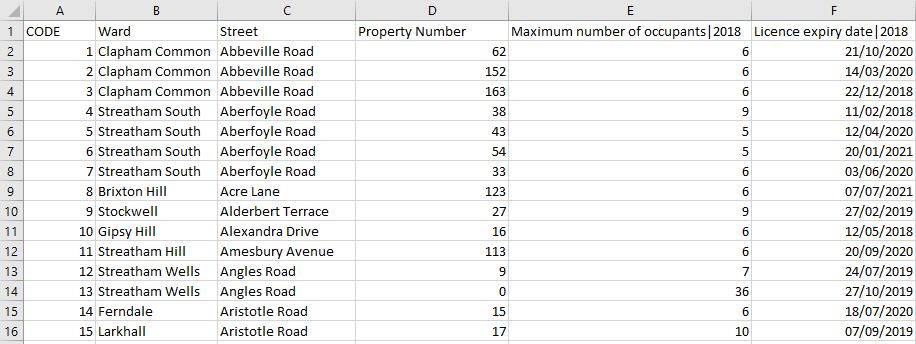
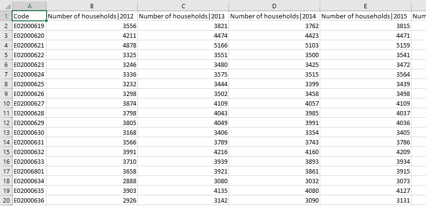
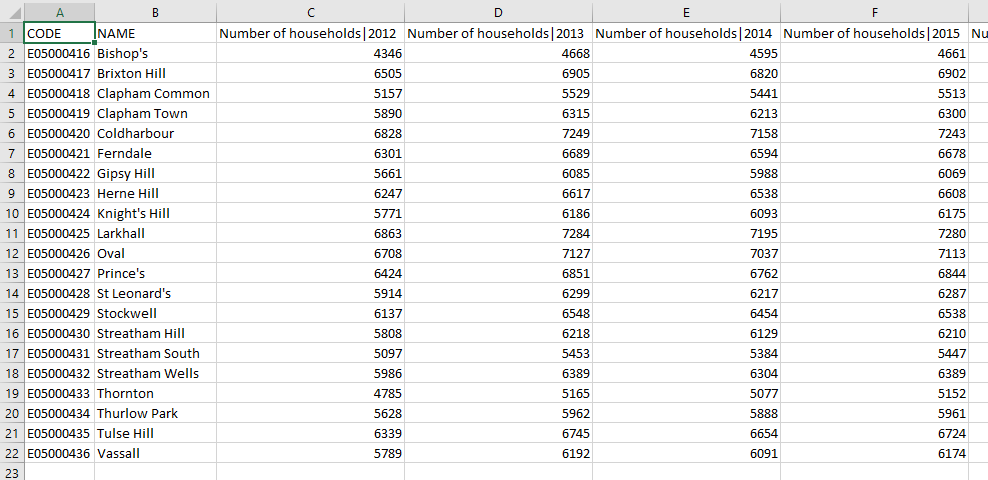
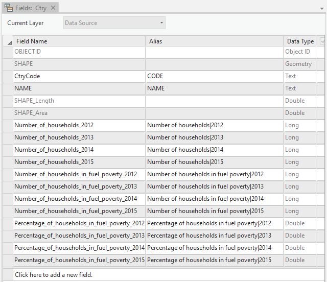
Now let’s have a look at the required format of the data you wish to load. The data needs to be in CSV format, one file per data layer. The first row needs to contain the column headers and each file needs to contain a column with the feature codes. These codes need to match the code column in the respective data layer in the file geodatabase so that you can connect the data to the data layers. The column headers should be specific enough to be unique and identifiable. To save having to rename the indicators later, it is advisable to enter the full indicator names into the column headers. You should also include the dates in the column headers, separated from the indicator name by a pipe character ‘|’. The dates should be sorted in ascending order. The image below shows the CSV file for the HMO data layer.
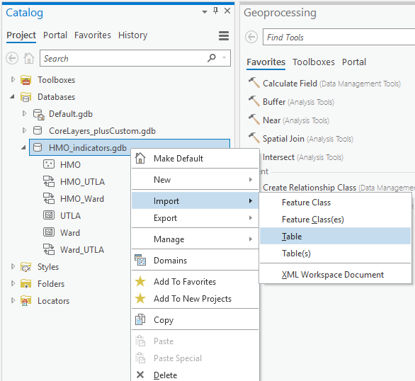
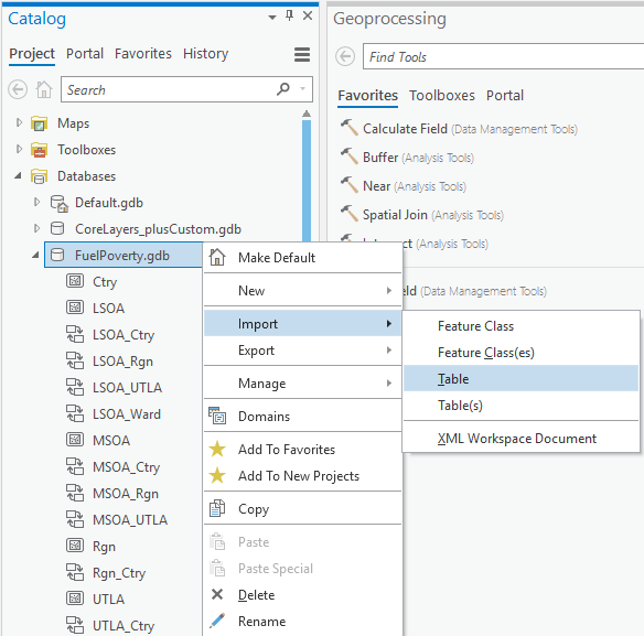
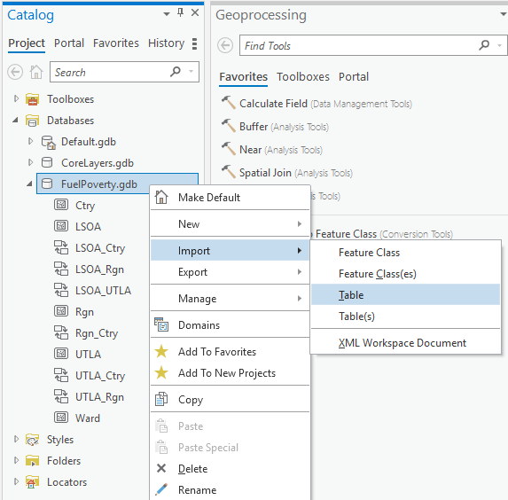
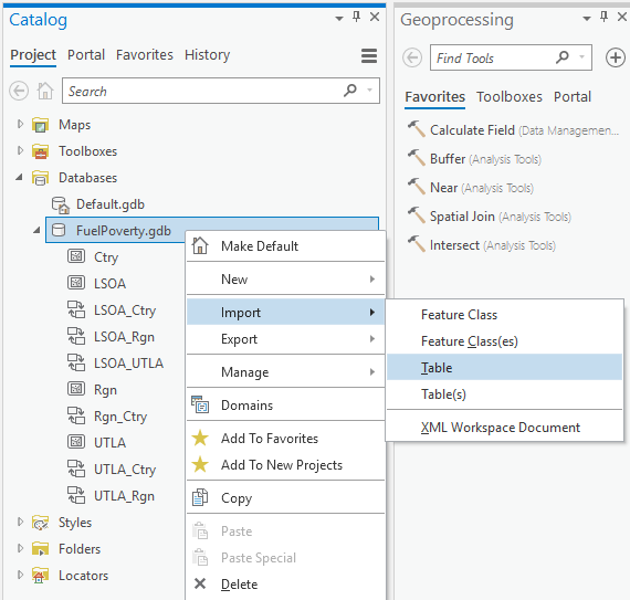
Now you can load the CSV files into your file geodatabase as tables. To do this, right-click on the database and select Import – Table.
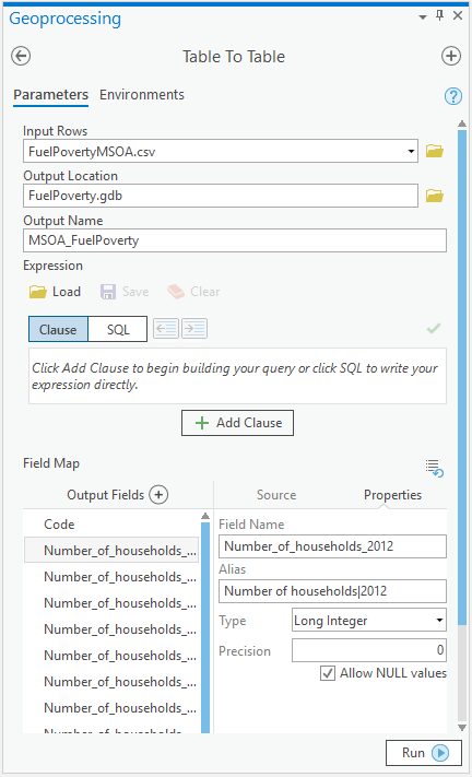
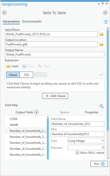
The Geoprocessing Tool Table To Table opens. Select one of the CSV files as Input Rows and give it a suitable Output Name (this table is just a temporary item in the database so the name does not matter).
It is now important to check that all of the output fields are loaded in the Field Map with their correct data type. Click on the first field and select Properties. The Type property is derived from the first value of the field so you should check that it is correct for each field and adjust if necessary. For example, if you add a rate indicator and the first value of the column happens to be an integer value, the whole field will be imported as Long Integer, stripping the decimal places from all other values of the column.
Click Run to import the data. When complete, the table will appear within your database in the Catalog Project pane. To check whether the import was successful, you can add the table to a map. You can open the table and see the values if you right-click on the entry in the Content pane and select Open.
Repeat the data loading steps for each of the CSV files.
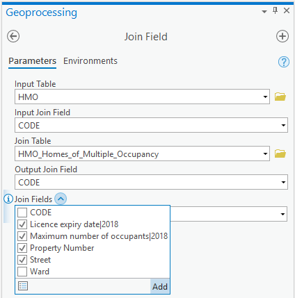
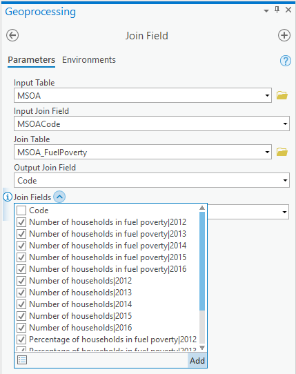
The next step is to join the data from the imported tables to the data layers. In the Geoprocessing pane, click the Back icon and find the tool called Join Field. Choose your data layer as the Input Table (you can drag and drop it from the Catalog Project pane) and the imported table as the Join Table. Select the matching code fields as Input and Output Join Field.
Open the Join Fields drop down and toggle all checkboxes to select all fields. There is a button at the bottom of the drop-down list that does this for you. You may wish to uncheck the columns containing the feature code and names as they will already exist in the data layer.
Then click Add and Run to join the selected fields to the data layer. The layer will automatically be added to your map if you have one open. You should check that the join was successful by opening the attribute table of the layer (right-click on the layer in the Content pane and select Attribute Table).
Once the joins are complete, you can delete the temporary tables you imported from the CSV files from the database (right-click on the item in the Catalog Project pane and select Delete).
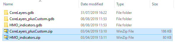
Now close ArcGIS Pro and browse to your file geodatabases in Windows explorer. Create a zip archive of the one containing the core layers including your new geography. You may wish to delete the ‘.gdb’ from the zip file name as this name will be the default name for the feature layer in ArcGIS Online.
Create another zip archive out of the file geodatabase containing the HMO indicators. Zip it and delete the ‘.gdb’ from the zip file name.
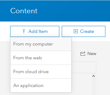
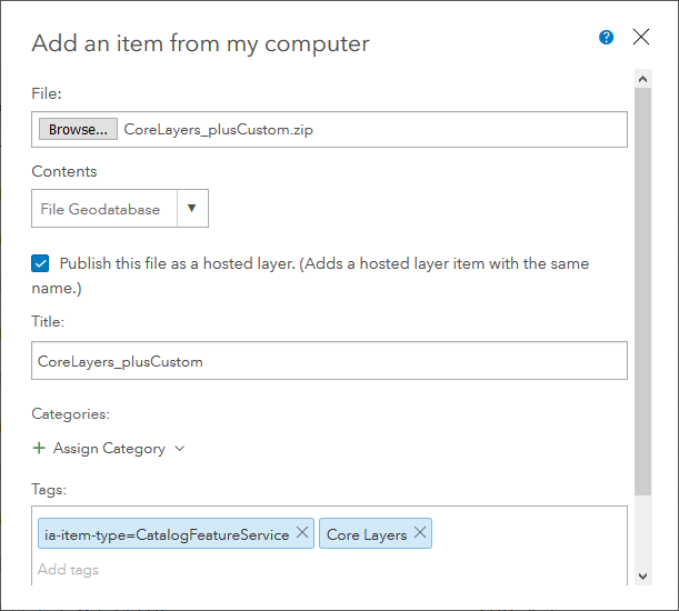
Back in ArcGIS Online, click on Content in the main menu and ensure the correct folder is selected. Then click on Add Item – From my computer and browse to the zipped file geodatabase containing the core layers including your new layer.
In the Contents drop down select File Geodatabase and keep the box for Publish this file as a hosted layer checked. You will have to add at least one tag called ia-item-type=CatalogFeatureService; this is essential for the comparsion areas to show in Dashbaord Builder and Report Builder. Feel free to add further tags (tags can help you find the item later through searches), then click Add Item.
Your file geodatabase is being converted to a feature layer and you will be redirected to its details page. Share the item with the Everyone (public) or with a specific group if you don’t want the data to be publicly visible. Please be aware that if you do not set it to be public, users will be asked to sign in to ArcGIS Online to see the data or any outputs that use it.
In the same way, upload and share the file geodatabase containing the indicator data as well.
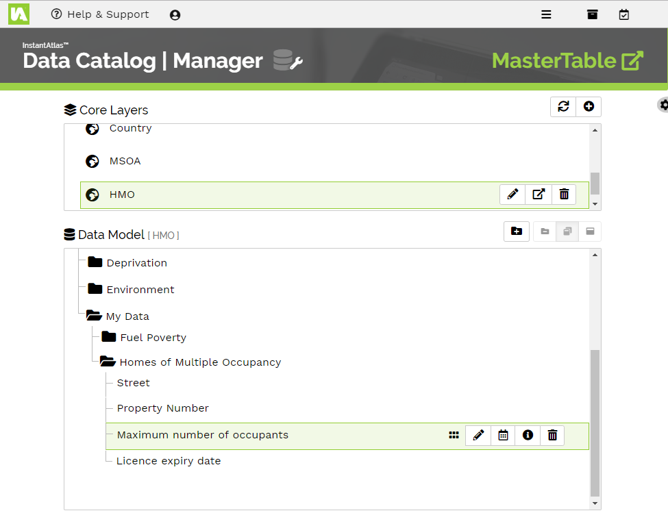
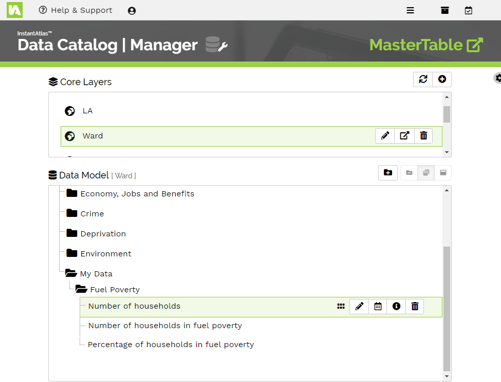
Now you should sign in to https://hub.instantatlas.com/ and click on the Manage Catalog button. You should see your Data Catalog with Core Layers and Data Model for each layer.
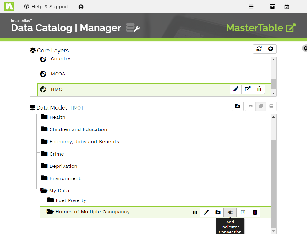
Click on the icon to the right of the core layers box to add further layers. Select the feature service you just added to ArcGIS Online containing your core layers. Select only the new layer you added (in this case the HMO layer)
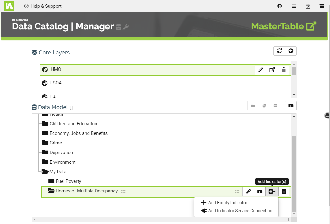
Select the HMO layer which will now appear at the bottom of your core layers list. You may wish to add a new theme and/or subtheme using the icon to the right of the data model. The theme hierarchy is the same for each core layer so you only need create a new theme once. Select the theme you wish to load the indicators into and click on the Add Indicator Connection button.
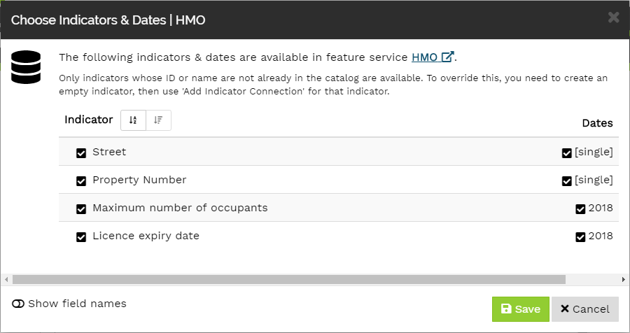
In the dialog that opens, select the feature layer with the indicator data you added to ArcGIS Online. If there are many feature layers in your organisation’s account you can use the search field or sort options at the bottom of the dialog to help you find the right one. Click Choose. Now select the correct layer that corresponds to the active core layer in your data catalog and click Choose. You will see a dialog with the fields you can add as indicators. Fields that have been formatted with a pipe character followed by a date are automatically recognised as different dates for the same indicator and will be pre-selected.
Select the indicator(s) you wish to add and click Save. The indicators should then appear in your data model.
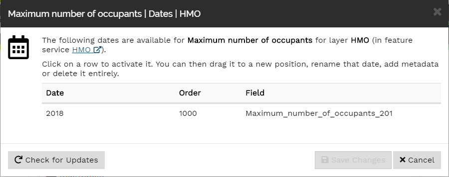
To check that the import was successful you can click on the icon to see the instances (dates) that are connected to the indicator.
Now import the indicators for the other core layers in the same way.
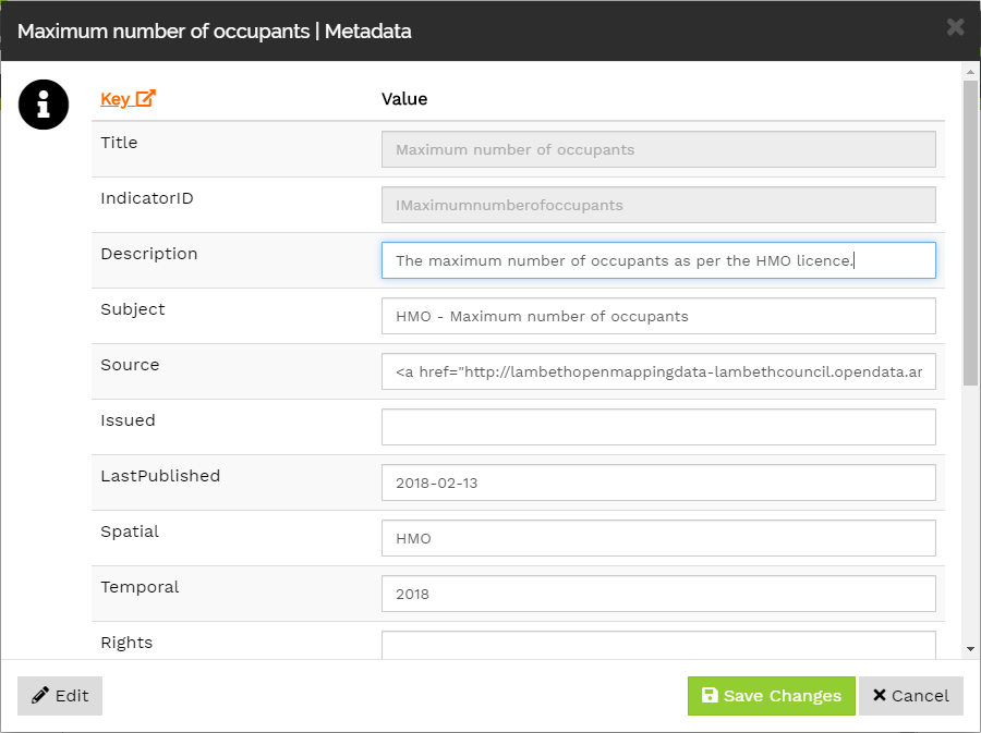
You can add metadata for the new indicators by clicking the icon and then clicking on the Edit button.
If you have a large number of indicators, adding metadata through the Data Catalog Manager interface may not be the most efficient method. As an alternative, you can create a CSV file containing the metadata for your new indicators and append it to your metadata table. Please contact support@instantatlas.com for information on how to do this.
Before carrying out any of the steps described below, we recommend that you read the full article to make sure that you have a clear understanding of the entire process. You should make a plan of what you need to do and note down the names that you want your geodatabases, hosted layers and fields to have. Think carefully about these and be consistent, as it may be difficult to change them later once you have created outputs (reports or dashboards) based on the new core layers and data. Contact support@instantatlas.com if you are unsure about anything before you start.
Let’s assume you previously loaded Fuel Poverty indicators into your data catalog and would now like to add data for these indicators for a layer that does not yet exist as a core layer in your data catalog, e.g. for MSOA. This article will explain the necessary steps to achieve this.
Please note that if you use one of the InstantAtlas National Data Services , you will not be able to add data to indicators managed by the data service. You can only add data to indicators you previously loaded yourself.
To add data into your data catalog, it needs to be saved in your ArcGIS Online account in one or more feature layers . If you want to use the data in either the Report Builder or Dashboard Builder apps, and you wish to see comparison values in the outputs, it is essential that the feature layers contain relationship classes between the core layers and also between the data layers. The Comparison Areas and Relationships page provides further information on this topic. At time of writing it is not possible to create relationship classes within ArcGIS Online so you will need to use either ArcGIS Pro or ArcMap to create the feature layer(s).
As you wish to add data for a new core layer you will need to have a shapefile containing the geometry (polygons, points or lines) for this layer. The shapefile must contain unique feature codes and names for the geography features in its attribute table. If you want to add relationship classes to use comparisons in Report Builder or Dashboard Builder, you will also need columns with lookups to the related layers in the attribute table of the shapefile.
To add data for new core layers to existing indicators you need to first locate the feature layer that the existing instances of this indicator are stored in. Data for all data layers of the same indicator must be saved in the same feature layer to be able to create the necessary relationship classes. The easiest way to find the feature layer is to open your data catalog in the Data Catalog Manager, find the indicator and click on the icon. At the top of the dialog you will see the link to the feature service.
Follow this link and you will see the layer description of the feature service. In the bread crumb at the top click on the item one level above. It will be called ‘something (FeatureServer)’.
On the feature server page, find the Service ItemId. Copy it to your clipboard.
Now sign in to your ArcGIS Online account and click on the magnifying glass in the main menu at the top to search for items. Paste the ID from your clipboard into the search field. As a result, you will see the feature layer that contains the fuel poverty indicators.
You can now either export the feature layer to a file geodatabase (open the item’s details page and click Export Data – Export to FGDB) or you can look for the file geodatabase that was used to originally create the feature layer. The latter would save the step of exporting but should only be done, if you are confident that the feature layer has not been changed since it was uploaded.
To find the file geodatabase from which the feature layer was originally created, open the details page of the feature layer and have a look at the Details section on the right underneath the buttons. Follow the link to the file geodatabase listed behind Created from.
From the details page of the File Geodatabase you can download the database using the Download button on the top right-hand side. Browse to the location you downloaded the database to and extract the zip archive.
When you received your master table and metadata table from the Geowise Support Team you would have also been sent a zip archive containing a file geodatabase with the core layers of your data catalog likely called <MyOrganisation>_CoreLayers.zip. If you have not received this, please contact support@instantatlas.com. This file geodatabase is a good starting point as it already contains the current core layers with their relationship classes. You should extract the zip archive and take a copy of the file geodatabase. Keep the original one as a reference and rename the copy to for example <MyOrganisation>_CoreLayers_plusCustom.gdb
Please note: We suggest that you add all of your custom core layers into the same file geodatabase, so if you are already using a feature layer called <MyOrganisation>_CoreLayers_plusCustom.gdb (or similar) in your data catalog you should find it in ArcGIS Online and download the respective file geodatabase.
Now open ArcGIS Pro and connect both file geodatabases (the one with the existing fuel poverty indicators and the one with the core layers) to your project. To do this, right-click on Databases in the Catalog Project pane and select Add Database. Then browse to the file geodatabase.
Firstly, you need to add the shapefile for your new core layer to the database with your core layers. To do this, right-click on the database name in the Catalog Project pane and select Import – Feature Class.
For the Input Features browse to the shapefile containing the new layer, enter a suitable Output Feature Class name and click Run.
Now add the relationship classes between the new layer and any other layers that apply. It is assumed that your shapefile contains the necessary lookup fields i.e. a column with the matching codes for each core layer that you want it to relate to. To create relationship classes, find the Geoprocessing Tool Create Relationship Class. Select the higher geography layer as Origin Table (e.g. UTLA) and lower geography layer as Destination Table (e.g. MSOA). You can drag and drop the layers from the database in the Catalog Project pane. The remaining properties will automatically get filled with default values. The ones you should change are:
Output Relationship Class: change the name to follow this pattern ‘<destination layer>_<origin layer>’ e.g. MSOA_UTLA. Please note that this is contrary to what ArcGIS Pro suggests by default!
Cardinality: change this to be One to many (1:M).
Origin Primary Key: Select the feature code field in the origin table.
Origin Foreign Key: Select the field in the destination table containing the matching codes from the origin table code field.
Leave all other settings on their default values and click Run. The relationship class will appear in your database. Create the relationship classes to other core layers in the same way.
If you want to use the new layer as comparison features for a lower-level geography, for example if you want to create a relationship between LSOA and MSOA, you will first need to add a column with the correct MSOA codes for each LSOA into the attribute table of the LSOA layer.
If you wish to add more than one new core layer to your data catalog, simply repeat the steps of importing a shapefile and creating the relevant relationship classes.
Now add the same layer and relationship classes to the fuel poverty database. As you want to add data to the layer within the fuel poverty database, you no longer call it core layer but data layer.
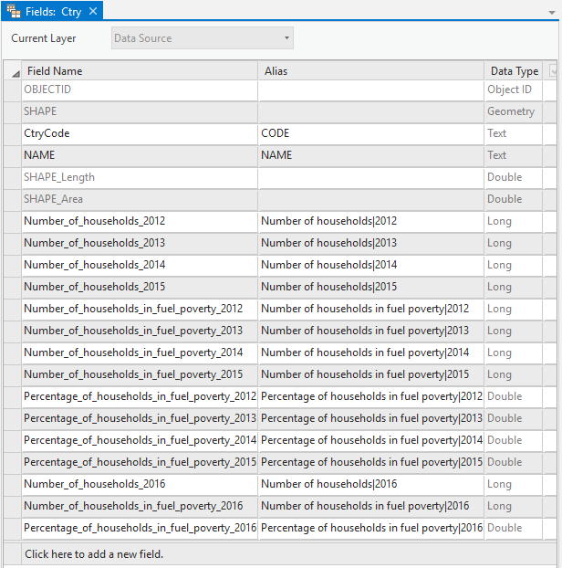
If you right-click on one of the data layers in your fuel poverty database (any except the new MSOA layer) and click on Design – Fields you will see the fields that are currently part of this layer. You can see the required field format for indicators with multiple dates in the Alias column: the indicator name needs to be followed by a pipe character ‘|’ and the date.
Before you can add the data for MSOA, you should ensure that it is correctly formatted. You will need one CSV file per data layer (in this example it would be just one file for the MSOA layer), containing a column with the geography feature codes. These codes need to match the code column in the respective data layer in the file geodatabase so that you can connect the data to the data layers. The first row needs to contain the column headers. The column headers of the indicator columns need to match those of the existing fields of the other layers, so that the Data Catalog Manager will understand that these are the same indicators, just for different layers.
If you wish to add data for multiple new core layers at the same time, you can do this in additional CSV files, applying the same rules.
Now you can load the CSV file into your File Geodatabase as a table. To do this, right-click on the database and select Import – Table.
The Geoprocessing Tool Table To Table opens. Select the CSV file as Input Rows and give it a suitable Output Name (this table is just a temporary item in the database so the name does not matter).
It is now important to check that all output fields are loaded in the Field Map with their correct data type. Click on the first field and select Properties. The Type property is derived from the first value of the field so you should check that it is correct for each field and adjust if necessary. For example, if you add a rate indicator and the first value of the column happens to be an integer value, the whole field will be imported as Long Integer, stripping the decimal places from all other values of the column.
Click Run to import the data. When complete, the table will appear within your database in the Catalog Project pane. To check whether the import was successful you can add the table to a map. You can open the table and see the values if you right-click on the entry in the Content pane and select Open.
Repeat the data loading steps for each of the CSV files if you are loading data for multiple data layers at a time.
The next step is to join the data from the imported table to the data layer. In the Geoprocessing pane, click the Back icon and find the tool called Join Field. Choose your data layer as the Input Table (you can drag and drop it from the Catalog Project pane) and the imported table as the Join Table. Select the matching code fields as Input and Output Join Field.
Open the Join Fields drop down and toggle all checkboxes to select all fields. There is a button at the bottom of the drop-down list that does this for you. You may wish to uncheck the columns containing the feature code and names as they will already exist in the data layer.
Then click Add and Run to join the selected fields to the data layer. The layer will automatically be added to your map if you have one open. You should check that the join was successful by opening the attribute table of the layer (right-click on the entry in the Content pane and select Attribute Table).
Once the join is complete you can delete the temporary table you imported from the CSV file from the database (right-click on the item in the Catalog Project pane and select Delete).
Now close ArcGIS Pro and browse to your file geodatabases in Windows explorer. Create a zip archive of the one containing the core layers including your new geography. You may wish to delete the ‘.gdb’ from the zip file name as this name will be the default name for the feature layer in ArcGIS Online.
Create another zip archive out of the file geodatabase containing the fuel poverty data. Ensure that the file name is the same as the zip archive you downloaded earlier from ArcGIS Online (if the original zip file is saved in the same folder and you want to keep it as a backup, you may wish to rename it first).
Back in ArcGIS Online, click on Content in the main menu and ensure the correct folder is selected. Then click on Add Item – From my computer and browse to the zipped file geodatabase containing the core layers including your new layer.
In the Contents drop down select File Geodatabase and keep the box for Publish this file as a hosted layer checked. You will have to add at least one tag called ia-item-type=CatalogFeatureService; this is essential for the comparsion areas to show in Dashbaord Builder and Report Builder. Feel free to add further tags (tags can help you find the item later through searches), then click Add Item.
Your file geodatabase is converted to a feature layer and you will be redirected to its details page. Share the item with the Everyone (public) or with a specific group if you don’t want the data to be publicly visible. Please be aware that if you do not set it to be public, users will be asked to sign in to ArcGIS Online to see the data or any outputs that use it.
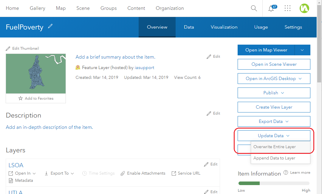
Now open the details page for the Fuel Poverty feature layer (note: not the related file geodatabase item!) and click on the Update Data button on the right. Then select the option Overwrite Entire Layer.
Browse to your zipped file geodatabase (the one you just added the MSOA data to) and click Overwrite. This will update the feature layer as well as the related file geodatabase.
Now you should sign in to https://hub.instantatlas.com/ and click on the Manage Catalog button. You should see your Data Catalog with Core Layers and Data Model for each layer.
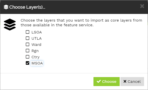
Click on the icon to the right of the core layers box to add further layers. Select the feature service you just added to ArcGIS Online containing your core layers. Select only the new layer you added (in this case the MSOA layer)
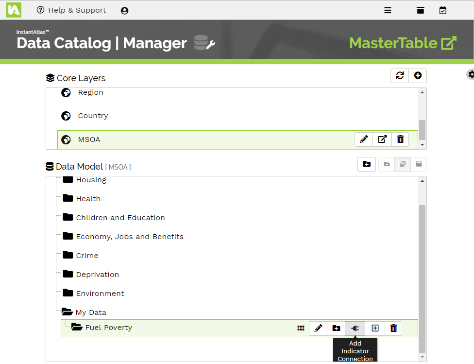
The MSOA layer will now appear at the bottom of your core layers list. Select the MOSA layer and expand the data model tree to the theme that contains the fuel poverty indicators in the other layers. Then click on the Add Indicator Connection button.
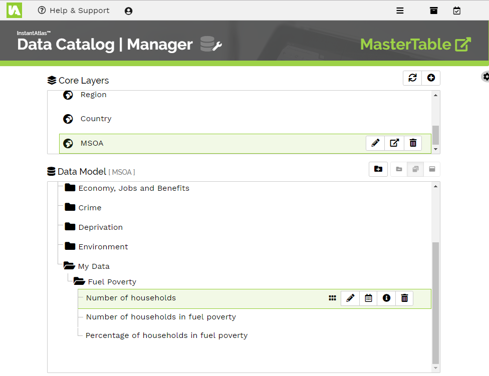
In the dialog that opens, select the feature layer with the fuel poverty data you updated in ArcGIS Online. If there are many feature layers in your organisation’s account you can use the search field or sort options at the bottom of the dialog to help you find the right one. Click Choose. Now select the correct data layer that corresponds to the active core layer in your data catalog and click OK. You will see a dialog with the fields you can add as indicators. Fields that have been formatted with a pipe character followed by a date are automatically recognised as different dates for the same indicator and will be pre-selected.
Select the indicator(s) you wish to add and click Save. The indicators should then appear in your data model.
To check that the import was successful you can click on the icon to see the instances (dates) that are connected to the indicator.
If you are adding data for multiple new core layers at a time you can now import the indicators for the other core layers in the same way.
You may wish to update the ‘Spatial’ metadata key (and maybe others) for the indicators to add the new core layer to the list. You can do this by clicking the icon and then clicking on the Edit button.
If you have a large number of indicators, adding metadata through the Data Catalog Manager interface may not be the most efficient method. As an alternative, you can create a CSV file containing the metadata for your new indicators and append it to your metadata table. Please contact support@instantatlas.com for information on how to do this.
Before carrying out any of the steps described below, we recommend that you read the full article to make sure that you have a clear understanding of the entire process. You should make a plan of what you need to do and note down the names that you want your geodatabases, hosted layers and fields to have. Think carefully about these and be consistent, as it may be difficult to change them later once you have created outputs (reports or dashboards) based on the new core layers and data. Contact support@instantatlas.com if you are unsure about anything before you start.
The data loading scenario for this article is the following: Your data catalog contains several core layers, e.g. LSOA, Wards, UTLA, Region and Country. You previously loaded your own Fuel Poverty indicators for a subset of these core layers (LSOA, UTLA, Region and Country) but not for the Ward layer. Now you would like to add data for these indicators for the Ward layer.
Please note that if you use one of the InstantAtlas National Data Services , you will not be able to add data to indicators that are part of the service. You can only add data to indicators you loaded yourself.
To add data into your data catalog, it needs to be saved in your ArcGIS Online account in one or more feature layers . If you want to use the data in either the Report Builder or Dashboard Builder apps, and you wish to see comparison values in the outputs, it is essential that the feature layers contain relationship classes between the core layers and also between the data layers. The Comparison Areas and Relationships page provides further information on this topic. At time of writing it is not possible to create relationship classes within ArcGIS Online so you will need to use either ArcGIS Pro or ArcMap to create the feature layer(s).
To add data to existing indicators for further core layers, you must first locate the feature layer that the existing instances of this indicator are stored in. Data for the same indicator across multiple layers must be saved in the same feature layer in order to be able to create the necessary relationship classes. The easiest way to find the feature layer is to open your data catalog in the Data Catalog Manager, find the indicator and click on the icon. At the top of the dialog you will see the link to the feature service.
Click this link and you will see the layer description of the feature service. In the bread crumb at the top click on the item one level above. It will be called ‘something (FeatureServer)’.
On the feature server page, find the Service ItemId. Copy it to your clipboard.
Now sign in to your ArcGIS Online account and click on the magnifying glass in the main menu at the top to search for items. Paste the ID from your clipboard into the search field. As a result, you will see the feature layer that contains the fuel poverty indicators.
You can now either export the feature layer to a file geodatabase (open the item’s details page and click Export Data – Export to FGDB) or you can look for the file geodatabase that was used to originally create the feature layer. The latter would save the step of exporting but should only be done, if you are confident that the feature layer has not been changed since it was uploaded.
To find the file geodatabase from which the feature layer was originally created, open the details page for the feature layer and have a look at the Details section on the right underneath the buttons. Follow the link to the file geodatabase listed next to Created from.
From the details page of the File Geodatabase you can download the database using the Download button on the top right-hand side. Browse to the location you downloaded the database to and extract the zip archive.
When you received your master table and metadata table from the Geowise Support Team you would have also been sent a zip archive containing a file geodatabase with the core layers of your data catalog likely called <MyOrganisation>_CoreLayers.zip. If you have not received this, please contact support@instantatlas.com. You will need this file geodatabase to get the Ward layer into the fuel poverty feature layer.
Now open ArcGIS Pro and connect both file geodatabases (the one with the existing fuel poverty indicators and the one with the core layers) to your project. To do this, right-click on Databases in the Catalog Project pane and select Add Database. Then browse to the file geodatabase.
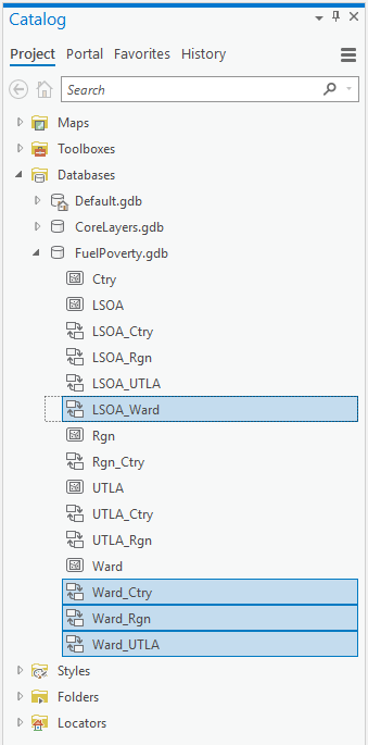
Expand the contents of both databases. You will see that the Ward layer only exists in the core layers database. To copy the layer to the fuel poverty database you should use the Geoprocessing Tool Feature Class to Feature Class. You can drag the Ward layer from the base core layers geodatabase into the Input Features field and drag the fuel poverty file geodatabase into the Output Location field. Give the Output Feature Class the same name as the input layer, in this case Ward.
Click Run and the Ward layer will be added to your fuel poverty database.
If you right-click on one of the data layers in your fuel poverty database (any layer except for the new Ward layer) and click on Design – Fields you will see the fields that are currently part of this layer. You can see the required field format for indicators with multiple dates in the Alias column: the indicator name needs to be followed by a pipe character ‘|’ and the date.
Before you can add the data for Wards, you should ensure that it is correctly formatted. You will need one CSV file per data layer (in this example it would be just one file for the Ward layer), containing a column with the feature codes. These codes need to match the code column in the respective data layer in the file geodatabase so that you can connect the data to the data layers. The first row needs to contain the column headers. The column headers of the indicator columns need to match those of the existing fields of the other data layers, so that the Data Catalog Manager will understand that these are the same indicators, just for different layers.
If you wish to add data for multiple existing core layers at the same time, you can do this in additional CSV files, applying the same rules.
Now you can load the CSV file into your File Geodatabase as a table. To do this, right-click on the database and select Import – Table.
The Geoprocessing Tool Table To Table opens. Select the CSV file as Input Rows and give it a suitable Output Name (this table is just a temporary item in the database so the name does not matter).
It is now important to check that all output fields are loaded in the Field Map with their correct data type. Click on the first field and select Properties. The Type property is derived from the first value of the field so you should check that it is correct for each field and adjust if necessary. For example, if you add a rate indicator and the first value of the column happens to be an integer value, the whole field will be imported as Long Integer, stripping the decimal places from all other values of the column.
Click Run to import the data. When complete, the table will appear within your database in the Catalog Project pane. To check whether the import was successful you can add the table to a map. You can open the table and see the values if you right-click on the entry in the Content pane and select Open.
Repeat the data loading steps for each of the CSV files if you are loading data for multiple layers at a time.
The next step is to join the data from the imported table to the data layer. In the Geoprocessing pane, click the Back icon and find the tool called Join Field. Choose your data layer as the Input Table (you can drag and drop it from the Catalog Project pane) and the imported table as the Join Table. Select the matching code fields as Input and Output Join Field.
Open the Join Fields drop down and toggle all checkboxes to select all fields. There is a button at the bottom of the drop-down list that does this for you. You may wish to uncheck the columns containing the feature code and names as they will already exist in the data layer.
Then click Add and Run to join the selected fields to the data layer. The layer will automatically be added to your map if you have one open. You should check that the join was successful by opening the attribute table of the layer (right-click on the layer in the Content pane and select Attribute Table).
Once the join is complete you can delete the temporary table you imported from the CSV file from the database (right-click on the item in the Catalog Project pane and select Delete).
To be able to see comparison geographies in a dashboard or report created with the InstantAtlas Dashboard Builder or InstantAtlas Report Builder apps respectively you will need relationship classes set up between the data layers in the underlying feature services. So far you have added the Ward layer to your fuel poverty file geodatabase, and have joined the data to the layer, but there are no relationship classes to other data layers yet.
To create relationship classes, find the Geoprocessing Tool Create Relationship Class. Select the higher data layer as Origin Table (e.g. UTLA) and the lower data layer as Destination Table (e.g. Ward). You can again drag and drop the layers from the fuel poverty database in the Catalog Project pane. The remaining properties will automatically be filled with default values. The ones you should change are:
Output Relationship Class: change the name to follow this pattern ‘<destination layer>_<origin layer>’ e.g. Ward_UTLA. Please note that this is contrary to what ArcGIS Pro suggests by default. You can add another underscore followed by a feature service identifier to the relationship class name e.g. Ward_UTLA_fuelpov.
Cardinality: change this to be One to many (1:M).
Origin Primary Key: Select the feature code field in the origin table.
Origin Foreign Key: Select the field in the destination table containing the matching codes from the origin table code field.
Leave all other settings at their default values and click Run. The relationship class will appear in your database. Create the relationship classes to other data layers in the same way.
Now close ArcGIS Pro and browse to your file geodatabase containing the fuel poverty data in Windows explorer. Zip it and ensure that the file name is the same as the zip archive you downloaded earlier from ArcGIS Online. If the original zip file is saved in the same folder and you want to keep it as a backup, you may wish to rename it first.
Back in ArcGIS Online, open the details page of the Fuel Poverty feature layer (not the related file geodatabase item) and click on the Update Data button on the right. Then select the option Overwrite Entire Layer.
Browse to your zipped file geodatabase (the one you just added the Ward data to) and click Overwrite. This will update the feature layer as well as the related file geodatabase.
Now you should sign in to https://hub.instantatlas.com/ and click on the Manage Catalog button. You should see your Data Catalog with Core Layers and Data Model for each layer.
Select the Ward layer and open the tree to the theme that contains the fuel poverty indicators in the other layers. Select the theme and click on the Add Indicator Connection button.
In the dialog that opens, select the feature layer you updated in ArcGIS Online. If there are many feature layers in your organisation’s account you can use the search field or sort options at the bottom of the dialog to help you find the right one. Click Choose. Now select the correct data layer that corresponds to the active core layer in your data catalog and click OK. You will see a dialog with the fields you can add as indicators. Fields that have been formatted with a pipe character followed by a date are automatically recognised as different dates for the same indicator and will be pre-selected.
Select the indicator(s) you wish to add and click Save. The indicators should then appear in your data model.
To check that the import was successful, you can click on the icon to see the instances (dates) belonging to the indicator.
If you are adding data for multiple core layers at a time you can now import the indicators for the other core layers in the same way.
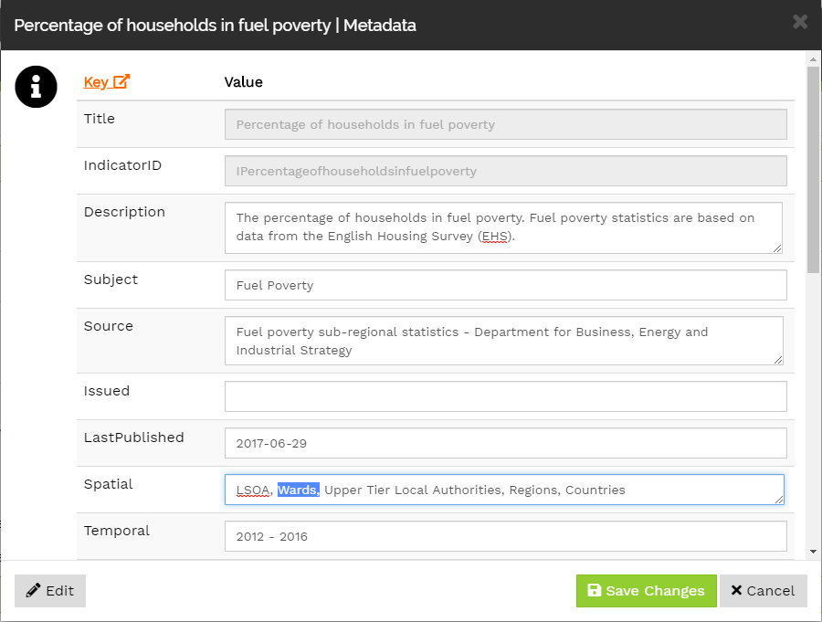
You may wish to update the ‘Spatial’ metadata key (and maybe others) for the indicators to add the new core layer to the list. You can do this by clicking the icon and then clicking on the Edit button.
If you have a large number of indicators, adding metadata through the Data Catalog Manager interface may not be the most efficient method. As an alternative, you can create a CSV file containing the metadata for your new indicators and append it to your metadata table. Please contact support@instantatlas.com for information on how to do this.
This article is particularly aimed at clients that use the InstantAtlas National Data Service and describes how to add a new date to existing indicators in a data catalog.
Before carrying out any of the steps described below, we recommend that you read the full article to make sure that you have a clear understanding of the entire process. You should make a plan of what you need to do and note down the names that you want your geodatabases, hosted layers and fields to have. Think carefully about these and be consistent, as it may be difficult to change them later once you have created outputs (reports or dashboards) based on the new core layers and data. Contact support@instantatlas.com if you are unsure about anything before you start.
Please note that if you use one of the InstantAtlas National Data Services , you will not be able to add dates to indicators that are part of the service. You can only add new dates to indicators you have loaded yourself.
For this example, let’s assume that you wish to load fuel poverty data for the year 2016 for LSOA, UTLA, Region and Country. The indicators already exist in your data catalog with the dates 2012 – 2015 for all four of these core layers.
To add new dates to existing indicators, you must first locate the feature layer that the existing instances are stored in. All dates for the same indicator must be saved in the same feature layer. The easiest way to find the feature layer is to open your data catalog in the Data Catalog Manager, find the indicator and click on the icon. At the top of the dialog you will see the link to the feature service.
Click this link and you will see the layer description of the feature service. In the bread crumb at the top click on the item one level above. It will be called ‘something (FeatureServer)’.
On the feature server page, find the Service ItemId. Copy it to your clipboard.
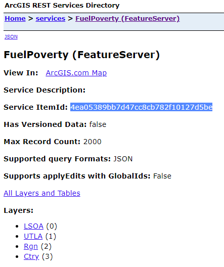
Now sign in to your ArcGIS Online account and click on the magnifying glass in the main menu at the top to search for items. Paste the ID from your clipboard into the search field. As a result, you will see the feature layer that contains the fuel poverty indicators.
You can now either export the feature layer to a file geodatabase (open the item’s details page and click Export Data – Export to FGDB) or you can look for the file geodatabase that was used to originally create the feature layer. The latter would save the step of exporting but should only be done, if you are confident that the feature layer has not been changed since it was uploaded.
To find the file geodatabase from which the feature layer was originally created, open the details page for the feature layer and have a look at the Details section on the right underneath the buttons. Follow the link to the file geodatabase listed next to Created from.
From the details page ofthe File Geodatabase, you can download the database using the Download button on the top right-hand side. Browse to the location you downloaded the database to and extract the zip archive.
Now open ArcGIS Pro and connect this file geodatabase to your project. To do this, right-click on Databases in the Catalog Project pane and select Add Database. Then browse to the file geodatabase.
Expand the contents of the database and you will see the four data layers with the fuel poverty data as well as the relationship classes between them. If you right-click on one of the data layers and click on Design – Fields you can see the fields that are currently part of this layer. You can see the required field format for indicators with multiple dates in the Alias column: the indicator name needs to be followed by a pipe character ‘|’ and the date.
Before you can add the data for 2016, you need to ensure that it is correctly formatted. You will need one CSV file per data layer. The first row needs to contain the column headers and each file needs to contain a column with the feature codes. These codes need to match the code column in the respective data layer in the file geodatabase so that you can connect the data to the data layers. The column headers of the indicator columns need to match those of the existing fields in the layer in ArcGIS Pro; only the date following the pipe character should be different.
If you wish to add multiple dates at the same time, you can do this in additional columns in the same file, applying the same rules.
Now you can load the CSV files into your File Geodatabase as a table. To do this, right-click on the database and select Import – Table.
The Geoprocessing Tool Table To Table opens. Select one of the CSV files as Input Rows and give it a suitable Output Name (this table is just a temporary item in the database so the name does not matter).
It is now important to check that all of the output fields are loaded in the Field Map with their correct data type. Click on the first field and select Properties. The Type property is derived from the first value of the field so you should check that it is correct for each field and adjust if necessary. For example, if you add a rate indicator and the first value of the column happens to be an integer value, the whole field will be imported as Long Integer, stripping the decimal places from all other values of the column.
Click Run to import the data. When complete, the table will appear within your database in the Catalog Project pane. To check whether the import was successful you can add the table to a map. You can open the table and see the values if you right-click on the layer in the Content pane and select Open.
Repeat the data loading steps for each of the CSV files.
The next step is to join the data from the imported tables to the data layers. In the Geoprocessing pane, click the Back icon and find the tool called Join Field. Choose your data layer as the Input Table (you can drag and drop it from the Catalog Project pane) and the imported table as the Join Table. Select the matching code fields as Input and Output Join Field.
Open the Join Fields drop down and toggle all checkboxes to select all fields. There is a button at the bottom of the drop-down list that does this for you. You may wish to uncheck the columns containing the feature code and names as they will already exist in the data layer.
Then click Add and Run to join the selected fields to the data layer. The layer will automatically be added to your map if you have one open. You should check that the join was successful by opening the attribute table of the layer (right-click on the layer in the Content pane and select Attribute Table).
Once the joins are complete, you can delete the temporary tables you imported from the CSV files from the database (right-click on the item in the Catalog Project pane and select Delete).
Now close ArcGIS Pro and browse to your file geodatabase in Windows explorer. Zip it and ensure that the file name is the same as the zip archive you downloaded earlier from ArcGIS Online. If the original zip file is saved in the same folder and you want to keep it as a backup, you may wish to rename it first.
Back in ArcGIS Online, open the details page of the Fuel Poverty feature layer (not the related file geodatabase item) and click on the Update Data button on the right. Then select the option Overwrite Entire Layer.
Browse to your zipped file geodatabase (the one you just added the 2016 data to) and click Overwrite. This will update the feature layer as well as the related file geodatabase.
Now you should sign in to https://hub.instantatlas.com/ and click on the Manage Catalog button. You should see your Data Catalog with Core Layers and Data Model for each layer.
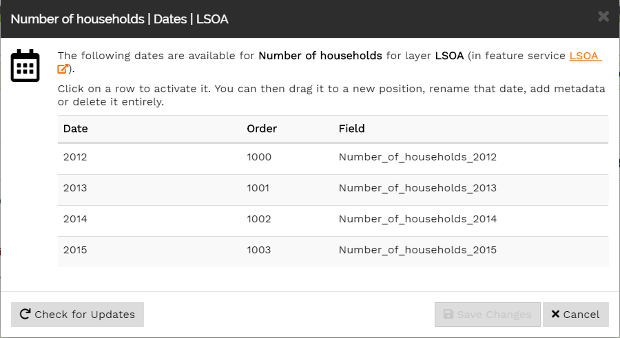
Select one of the core layers that has data for Fuel Poverty, e.g. LSOA and find the indicators in the tree.
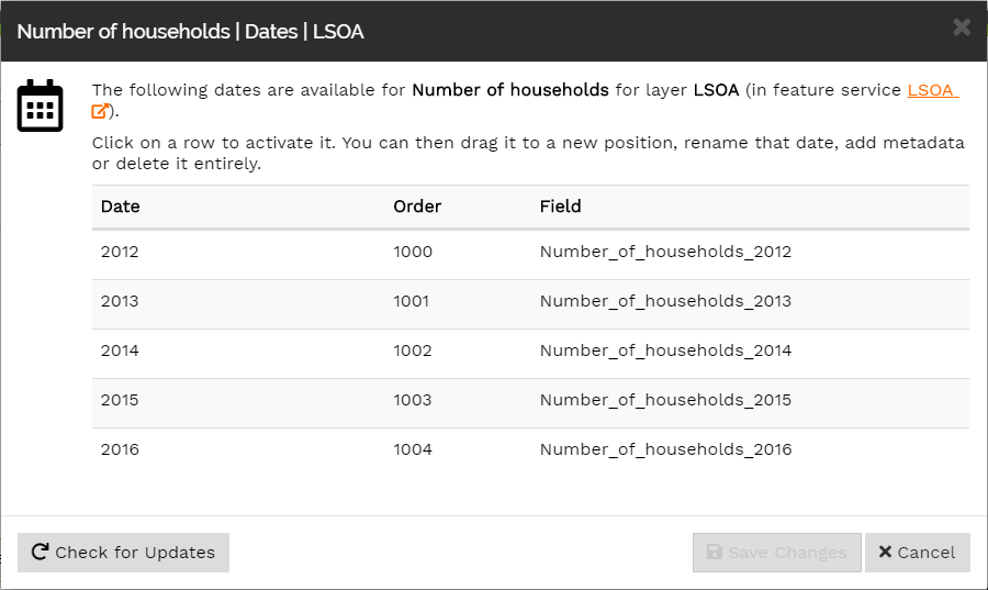
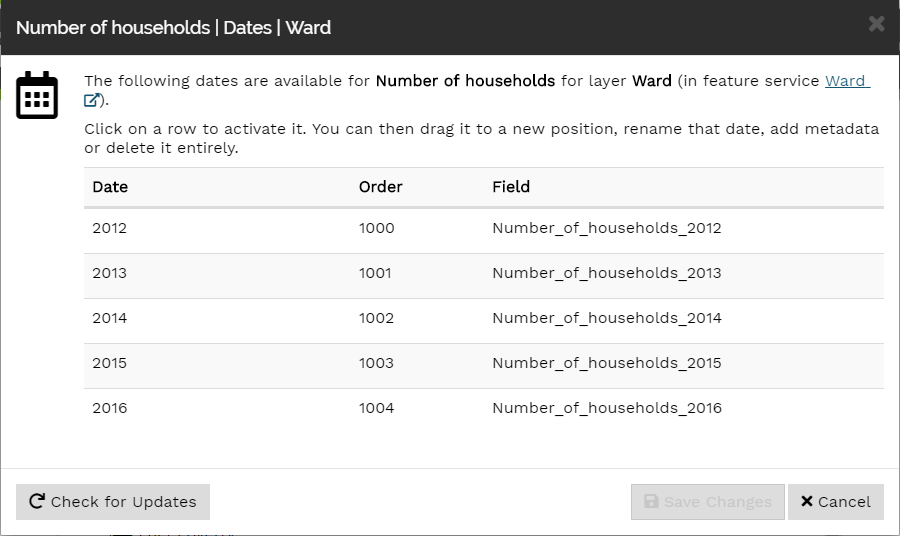
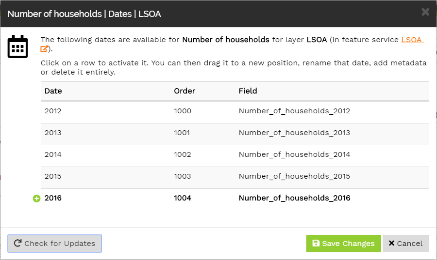
Click on the icon for one of the indicators and then click the Check for Updates button in the bottom left corner of the Dates dialog. The Data Catalog Manager will find 2016 as a new date for the indicator.
Click Save Changes to confirm that you wish to add the new date.
You should now repeat the Check for Update step for each indicator of each core layer for this dataset.
You may wish to update the ‘Temporal’ metadata key (and maybe others) for the indicators to add the new date to the range. You can do this by clicking the icon and then clicking on the Edit button.
If you have a large number of indicators, adding metadata through the Data Catalog Manager interface may not be the most efficient method. As an alternative, you can create a CSV file containing the metadata for your new indicators and append it to your metadata table. Please contact support@instantatlas.com for information on how to do this.


