In addition to the ‘Geography and Filters’ worksheet, you must have at least one datasheet in your workbook. Datasheets are where you enter the actual data values that will ultimately be displayed in your report. A worksheet becomes an active datasheet when its name starts with ‘iadatasheet’. To rename a worksheet in Excel, you simply right click on the worksheet name and select ‘Rename’. You can put all of your data values in one datasheet or spread them between two or more datasheets.

Your workbook can contain one or more active datasheets. Note that worksheet names must be unique in Excel. So if your workbook contains more than one active datasheet you could, for example, name them iadatasheet1, iadatasheet2, iadatasheet3 and so on. The number of active datasheets will affect the number of data files produced when the data is exported – this will be explained in more detail in section ‘Exporting Data Files’.

Entering Indicators

Please refer to the ‘Example 1 iadatasheet’ of the example workbook.

Entering Codes (Column A)

The contents of this column must be exactly the same as that of column A in the ‘Geography and Filters’ worksheet.

Entering Names (Column B)

The contents of this column must be exactly the same as that of column B in the ‘Geography and Filters’ worksheet.

Entering Indicator Values (Columns C Onwards)

Columns C onwards hold the data values that will be displayed in your report. The data you enter must be organised on three levels: by theme, by indicator and by time period.

Rows 1 and 2
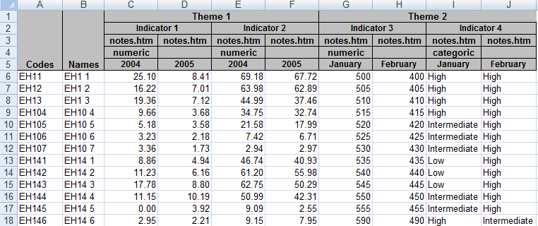
Row 1 contains the theme names, row 2 the indicator names. These names can be anything you like. Be careful not to include leading or trailing spaces as these may result in errors in an InstantAtlas report.

You can see that the cells in rows 1 and 2 are merged so that they span more than one column. This is because the cell containing a theme name must span all the columns belonging to that theme. Similarly, the cell containing an indicator name must span all the columns belonging to that indicator. It is very important that cells containing theme and indicator names span the correct number of columns or the data files you generate will be invalid.

There are two time periods with data for Indicator 1: 2004 and 2005. Thus the cell containing the indicator name must span two columns. There are two indicators in Theme 1, each with two columns containing data. Thus the cell containing the theme name must span four columns.

In an Excel worksheet, one cell can be made to span a number of columns by merging. You can merge cells in a spreadsheet by doing the following:

1. Select the cells you want to merge by clicking and dragging so that they are highlighted
2. Right-click your selection
3. Choose Format Cells… from the context menu.
4. Click the Alignment tab
5. Tick the box labelled Merge cells
6. Click OK

Row 3
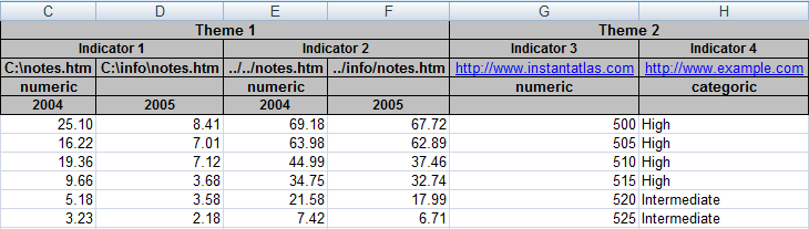
Row 3 is used to provide links to files of your choice. These are the files that will open when the notes icon for an indicator or time period (lowest hierarchy level) is clicked in the data explorer of a report. This is usually used to link to indicator-related metadata. You can specify a different link for each indicator or time period.

In the example workbook, ‘notes.htm’ has been entered for every indicator. This means that when the notes button is clicked, a file called ‘notes.htm’ located in the report folder will open. You can type in any links you like. The pathnames you enter can be absolute or relative. The following image shows examples of some alternative links that you might enter.

Row 4
Row 4 is used to specify the type of indicator. This can be ‘numeric’ or ‘categoric’. You only need to specify the indicator type in the first column for each indicator.

Indicator Type	numeric	categoric
Use when…	…the data values for your indicator are numerical.	…the data values for your indicator are textual rather than numerical.
Sorting in Data Table	numerical	alphabetical
Alignment in Data Table	right aligned	left aligned
Examples	The percentage of population in the 15-18 age group or average household income	Political affiliation (Republican, Democrat, etc) or land classification (Urban, Rural, etc)

It is possible to specify a precision value in the metadata for numeric indicators. For ‘categoric’ indicator types, this precision value is ignored.

Row 5
Row 5 contains the time period names. These names can be anything you like. Time periods for an indicator should be entered in columns from left to right in ascending chronological order. If you only have a single time period for each indicator, you can leave the cells in row 5 blank. You will then just see two levels (Theme >> Indicator) instead of three (Theme >> Indicator >> Time Period) in the data explorer of your report.

Data values
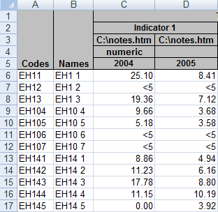
Starting in cell C6 you should enter your data values. As indicated above, you should generally enter numbers for ‘numeric’ type indicators and text values for ‘categoric’ type indicators. However, it is possible to enter text values for ‘numeric’ type indicators – this can be useful if, for example, you need to suppress a value due to a case of small numbers. In the following image you can see that <5 has been entered as a data value for three geographic features. This is a text value and will be treated as such – these areas will be classified separately by the legend. Other text values used for ‘numeric’ type indicators might be ‘-’ or ‘N/A’ for example.

You do not have to enter a data value for every geographic feature – if you leave a cell blank then “No Data” (or some other text you set in the configuration file of the report using the InstantAtlas Designer) will be displayed in the report for this area. In the example workbook, data values have not been entered for three features in the base geography.

The Data Manager must not contain any Excel error codes such as ‘#DIV/0!’. These error codes may be present if values in the worksheet are the result of a formula. The result of formulas can be used to generate data though it is considered safer to copy and paste these as ‘values’.

The dynamic report will show your numbers with a thousand separator symbol accoding to the number local setting in the config.xml file, editable through the InstantAtlas Designer. However, numbers in Excel should not have a thousand place separator (e.g. 12,000).  If they do have one e.g a comma, point or thin space, you can change this by doing the following:

1. Select the range of cells containing the data values so that they are highlighted
2. Right-click and select ‘Format Cells…’ from the context menu
3. n the ‘Format Cells’ dialog, in the ‘Number’ tab, ensure the ‘Use 1000 Separator’ checkbox is not checked. Click ‘OK’.

InstantAtlas reports will by default display your data values with the decimal places setting for the cells in your workbook. To change the number of decimal places you can do the following:

1. Select the range of cells containing the data values so that they are highlighted
2. Right-click and select ‘Format Cells…’ from the context menu
3. In the ‘Format Cells’ dialog, in the ‘Number’ tab, ensure the ‘Category’ is set to ‘Number’ and then edit the number of decimal places. Click ‘OK’.

We recommend that you avoid data values with excessive precision (7.34167683947). There are two main considerations when you choose the number of decimal places for an indicator:

1. The number of decimal places necessary for interpretation by the end-user of the dynamic report (long numbers are more difficult to visualise/interpret)
2. The performance of the dynamic report (long numbers mean larger data files and potentially a reduction in the speed of the report)

You should round values with an excessive number of decimal places as described above.

Adding further themes/indicators/time periods
Simply add further data in the columns to the right of the existing data. Make sure you enter the names, links, indicator type and time period labels in rows 1-5 and that you merge cells in rows 1-2 as required. If you run out of columns (the limit in Excel 97-2003 is 255, from Excel 2007 onwards the limit is 16,384 columns), simply do the following:

1. Insert a new worksheet into your workbook
2. Copy columns A and B from the previous worksheet
3. Paste the contents into columns A and B of your new worksheet
4. Start adding data in columns C onwards
5. Rename the worksheet to a name starting with ‘iadatasheet’ to make it an active datasheet

Please note that you cannot split a theme over two or more datasheets, so the new datasheet needs to start with a new theme.

Entering Associate Values

Please refer to the ‘Example 2 iadatasheet’ of the example workbook.
An associate is a set of values that are so called because they are associated to indicator values. Associate values are not unsually used in thematic mapping in InstantAtlas reports but perform other roles. The inclusion of associate values is optional but the default configuration of some templates assumes that you will be supplying certain associates. The table below lists these associates.

Associate	Reason for including in your data file(s)
ll	Lower confidence limits are displayed as error bars in a report bar chart. You can calculate these confidence limits in any way you like.
ul	Upper confidence limits are displayed as error bars in a report bar chart. You can calculate these confidence limits in any way you like.
largestObservation, upperQuartile, median, lowerQuartile, smallestObservation	These associates need to be provided if you would like to use the box-and-whisker chart in your report. This chart can be included in the Single Map template using the Designer.
diff, number, significance, baseline, state, trend, target	These associates perform various roles in the Area Profile template. For more information please refer to section ‘The InstantAtlas Area Profile Template’.
xValue, yValue, sizeValue, denominator, numerator	These associates perform various roles in the Scatter Plot template. For more information please refer to section ‘The InstantAtlas Scatter Plot Template’.

In addition to those listed in the table above you can supply your own associates. You will need to configure your dynamic report using the InstantAtlas Designer to make use of any custom associate(s) you have supplied. Typically this is done by adding an extra column to the data table and linking this new column to the custom associate (the column name must match the associate name). You can also use associates to populate the Area Breakdown Pie Chart.

The ‘Example 2 iadatasheet’ worksheet demonstrates how to include associate values in your workbook. Associate values are entered in columns directly to the right of the indicator values to which they relate. Note that you do not have to supply the same set of associates for every date or indicator – you might decide to enter these for some but not others.

You must merge cells in row 3 to tell InstantAtlas which columns belong to each time period instance of an indicator. Associates should be named in row 5 as in the table above. Associate names must be consistent across dates/indicators. Note that these are not the names displayed in an InstantAtlas report – the report will display an alias that you can configure using the InstantAtlas Designer. If you supply your own custom associates, we recommend you keep the associate name simple (i.e. a single word that does not include any special characters).

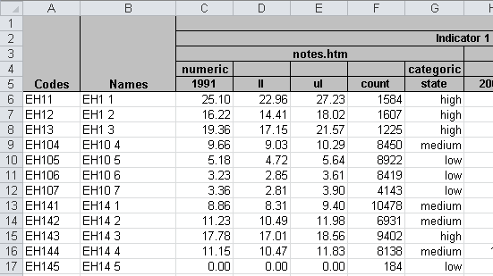
The ‘count’ and ‘state’ associates in the ‘Example 2 iadatasheet’ worksheet are examples of custom associates that can be added. When mapping rates it is good practice to show counts alongside them in the data table. You can add a ‘Count’ column to the data table of your report using the InstantAtlas Designer and configure it to pick up an associate in the data file called ‘count’ (see ‘ Table Properties’ for more information). The same applies to the ‘state’ associate respectively.

By default associate columns are assumed to be of type numeric. If you have associate columns with textual data you should change the type to be categoric. You can do this either in the iadatasheet in the cell directly above the associate column name (row 4) or alternatively you can define the type in the ‘Metadata’ worksheet. Please refer to section ‘Setting a Data Type for Associates’ for further information.